MATLAB to optimise the stalagmite function and find the global maxima of the function

Aim: Use MATLAB to optimise the stalagmite function and find the global maxima of the function.

Governing equations:

Stalagmite function

f(x,y) = f_1.x* f_2.x * f_1.y * f_2.x

f_1.x = [sin(5.1πx + 0.5)]⁶

f_1.y = [sin(5.1πy + 0.5)]⁶

f_2.x = exp[-4ln(2)(x-0.0667)^2/0.64]

f_2.y = exp[-4ln(2)(x-0.0667)^2/0.64]

Objectives:

1. To optimise the stalagmite function.
2. To find global maxima.
3. To find the optimum input values.

Body:

Stalagmite and Stalactite

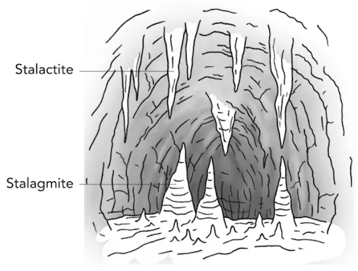
Stalactites are structures formed from mineral deposits that hang from caves. These formations hold tightly to the ceiling and hang down. As opposed to hanging from the ceiling, Stalagmite structures are formed from the cave floor that point upward. Stalagmite and Stalactite functions are mathematical functions which represents shapes similar to that of the stalagmite and stalactite functions.

Genetic Algorithm

A genetic algorithm is a search heuristic that's inspired by Charles Darwin’s theory of natural evolution. This algorithm reflects the method of survival where the fittest individuals are selected for reproduction so as to supply offspring of subsequent generation.

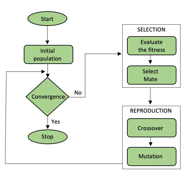
Initial population - The process begins with a set of individuals which is called a Population. Each individual is a solution to the problem we want to solve.An individual is characterized by a set of parameters (variables) known as Genes. Genes are joined into a string to form a Chromosome (solution) and set of the individuals are called population.

Convergence - The algorithm terminates if the population has converged (does not produce offspring which are significantly different from the previous generation). Then it's said that the genetic algorithm has provided a group of solutions to our problem.

Fitness function - The fitness function determines how fit a private is (the ability of a private to compete with other individuals). It gives a fitness score to every individual. The probability that a private are going to be selected for copy is predicated on its fitness score.

Crossover - Crossover is that the most vital introduce a genetic algorithm. for every pair of oldsters to be mated, a crossover point is chosen randomly from within the genes.

Mutation - In certain new offspring formed, a number of their genes are often subjected to a mutation with a coffee random probability. this suggests that a number of the bits within the bit string are often flipped.

Genetic algorithm in MATLAB:

Syntax - [input, f] = ga(fun, nvars, A, b, Aeq, beq, lb, ub, nonlcon, options) minimizes with the default optimization parameters replaced by values in options. (Set nonlcon=[] if no nonlinear constraints exist.).

fun = @function

nvars = number of variables

subject to the linear inequalities A*x ≤ b. ga evaluates the matrix product A*x as if x is transposed (A*x').

nonlcon = nonlinear constraints

options = can be used such as population size etc with the help of optimoptions

MATLAB code:

clear all
close all
clc

% Defining our search space
x = linspace(0,0.6,150);
y = linspace(0,0.6,150);

iteratinon_limit = 50;

% Creating a 2Dimensional mesh
[xx,yy] = meshgrid(x,y);


% Evaluating the stalagmite function 

for i=1:length(xx)
    for j=1:length(yy)
        input_vector(1)=xx(i,j);
        input_vector(2)=yy(i,j);
       f(i,j)= stalagmite(input_vector);
    end
end

% Case-1 Unbound

tic 
for i=1:iteratinon_limit

[input,fopt(i)]=ga(@stalagmite_fun,2);

x_out(i)=input(1);
y_out(i)=input(2);

end

case_1_time = toc

figure('name','Unbound')
subplot(2,1,1)
surfc(x,y,-f)
xlabel('x');
ylabel('y');
title('Case-1 Unbounded ','color','k');
shading interp
hold on
plot3(x_out,y_out,-fopt,'marker','o','markersize',6,'markerfacecolor','r');
subplot(2,1,2)
plot(-fopt);
xlabel('No Of Iterations');
ylabel('max Function Value');

% Case-2 bounded

tic 
for i=1:iteratinon_limit

[input,fopt(i)]=ga(@stalagmite_fun,2,[],[],[],[],[0,0],[0.6,0.6]);

x_out(i)=input(1);
y_out(i)=input(2);

end

case_2_time = toc

figure('name','bounded')

subplot(2,1,1)
surfc(x,y,-f)
xlabel('x');
ylabel('y');
title('Case-2 bounded ','color','k');
shading interp
hold on
plot3(x_out,y_out,-fopt,'marker','o','markersize',6,'markerfacecolor','r');
subplot(2,1,2)
plot(-fopt);
xlabel('No Of Iterations');
ylabel('max Function Value');

% case-3 Fixed population of 150

options = optimoptions('ga');
options = optimoptions(options,'populationsize',150);

tic 
for i=1:iteratinon_limit

[input,fopt(i)]=ga(@stalagmite_fun,2,[],[],[],[],[0,0],[0.6,0.6],[],[],options);

x_out(i)=input(1);
y_out(i)=input(2);

end

case_3_time = toc

figure('name','bounded fixed population')

subplot(2,1,1)
surfc(x,y,-f)
xlabel('x');
ylabel('y');
title('Case-3 fixed population ','color','k');
shading interp
hold on
plot3(x_out,y_out,-fopt,'marker','o','markersize',6,'markerfacecolor','r');
subplot(2,1,2)
plot(-fopt);
xlabel('No Of Iterations');
ylabel('max Function Value');

% case-4 Fixed population of 300

options = optimoptions('ga');
options = optimoptions(options,'populationsize',300);

tic 
for i=1:iteratinon_limit

[input,fopt(i)]=ga(@stalagmite_fun,2,[],[],[],[],[0,0],[0.6,0.6],[],[],options);

x_out(i)=input(1);
y_out(i)=input(2);

end

case_4_time = toc

figure('name','bounded fixed population 300')

subplot(2,1,1)
surfc(x,y,-f)
xlabel('x');
ylabel('y');
title('Case-4 fixed population 300','color','k');
shading interp
hold on
plot3(x_out,y_out,-fopt,'marker','o','markersize',6,'markerfacecolor','r');
subplot(2,1,2)
plot(-fopt);
xlabel('No Of Iterations');
ylabel('max Function Value');
display(input)

% End of the program

Explanation:

Lines 5-12

x and y inputs are defined and 2D mesh grid is created.

Lines 15-23

Nested for loop is used to create input vector which is then passed to a separate function -fitness function defined by us as stalagmite function and the value of the function is calculated.

Lines 25-51

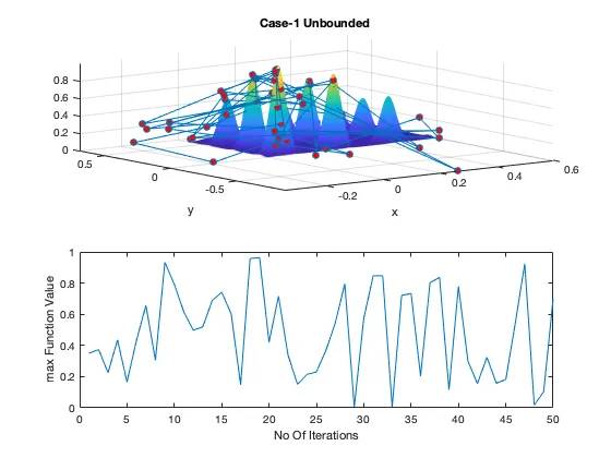
Case-1, in this the values of x and y are unbounded i.e. it can take values below the defined value, Iteration limit is set and tic-toc command is used to calculate the time required to calculate the amount of time required to complete the process.

subplot is used to plot the surface plot and plot( fopt ) on the same figure.

Lines 53-80

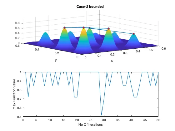
Case-2, in this the values of x and y are bounded i.e. it can take values between 0 & 0.6, Iteration limit is set and tic-toc command is used to calculate the time required to calculate the amount of time required to complete the process.

subplot is used to plot the surface plot and plot( fopt ) on the same figure.

Lines 82-112

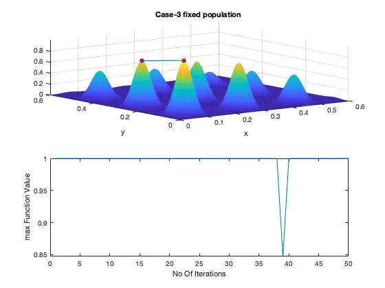
Case-3, in this the values of x and y are bounded i.e. it can take values between 0 & 0.6, options command is used to set the population count to 150 ,Iteration limit is set and tic-toc command is used to calculate the time required to calculate the amount of time required to complete the process.

subplot is used to plot the surface plot and plot( fopt ) on the same figure.

Lines 114-145

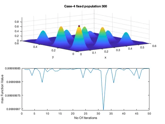
Case-4, in this the values of x and y are bounded i.e. it can take values between 0 & 0.6, options command is used to set the population count to 300 ,Iteration limit is set and tic-toc command is used to calculate the time required to calculate the amount of time required to complete the process.

subplot is used to plot the surface plot and plot( fopt ) on the same figure.

Function:

function [f]= stalagmite(input_vector)

f1x= (sin((5.1*pi).*input_vector(1)+0.5)).^6;
f1y= (sin((5.1*pi).*input_vector(2)+0.5)).^6;

f2x= exp((((input_vector(1)-0.0667).^2)/0.64).*(-4*log(2)));
f2y= exp((((input_vector(2)-0.0667).^2)/0.64).*(-4*log(2)));
f1=f1x*f1y*f2x*f2y;
f=-f1;
end

Explanation:

The function takes input vector generated in line 17 as input and return the function value.

Result:

1. Unbounded i.e. the input values can go beyond the defined range.

2. Bounded i.e. the input value ranges only in the defined range.

3. Bounded with the population size of 150.

4. Bounded with the population size of 300.

Conclusion:

In many problems we are often required to optimise the functions as to get the optimum solutions of the problem out of all the available solutions hence the study of Genetic algorithm is of great importance in the field of engineering.

Sources:

https://in.mathworks.com/discovery/genetic-algorithm.html

https://in.mathworks.com/help/gads/ga.html

https://in.mathworks.com/help/optim/ug/optim.problemdef.optimizationproblem.optimoptions.html