Challenge

Parsing NASA thermodynamic data

GGulshan Kumar16 Nov 2020

MATLAB

AIM: Writing the MATLAB program to Parse NASA thermodynamic data and calculating thermodynamic properties.

GOVERNING EQUATION:

Where,

Cp = Specific heat

H = Enthalpy

S = Entropy

R = Universal gas constant

OBJECTIVES:

Write a function that extracts the 14 co-efficient and calculates the enthalpy, entropy, and specific heats for all the species in the data file.
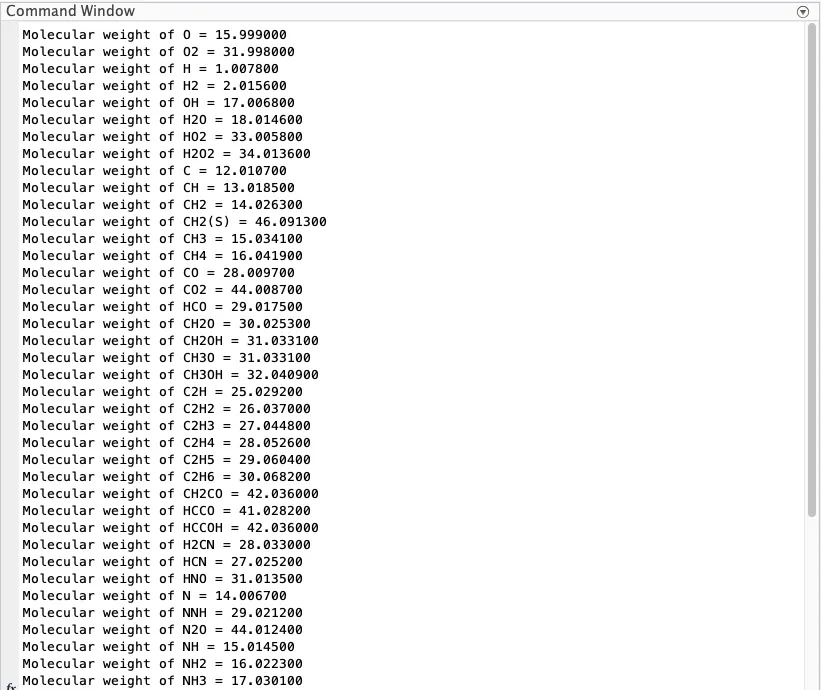
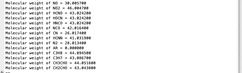
Calculate the molecular weight of each species and display it in the command window.
Plot the Cp, Enthalpy, and Entropy for the local temperature range (low temperature: high temperature) specific for each species.
The main program will just take the "THERMO.dat" file as an input and generate Cp, H, and S plots.
Save the plots as images with appropriate names and dump them in separate folders for each species with a suitable name. All of these should be generated automatically.
Generating Cp, H, and S plots for o2, N2, and Co2 species.

BODY:

NASA came up with polynomials that can be used to evaluate thermodynamic properties such as Cp, H, and S. They have also documented the co-efficient that are required to evaluate these polynomials for 1000+ species, the file “THERMO.dat” contains such data for 53 species.

Our work is to calculate the thermodynamic properties and generate appropriate plots.

Lets first look into these thermodynamic properties.

1. Specific Heat

In thermodynamics, the specific heat capacity (symbol Cp) of a substance is the heat capacity of a sample of the substance divided by the mass of the sample. Informally, it is the amount of energy that must be added, in the form of heat, to one unit of mass of the substance in order to cause an increase of one unit in temperature. The SI unit of specific heat is joule per kelvin and kilogram, J/(K kg).

Specific heat for different substance varies with temperature and the variation is given by the relation.

By plugging appropriate values of the coefficients in the above equation we can calculate the variation of specific heat for species such as oxygen, nitrogen etc w.r.t temperature.

2. Entropy

It is a property of thermodynamic system. The term entropy was introduced by Rudolf Clausius who named it from the Greek word τρoπή, "transformation". He considered transfers of energy as heat and work between bodies of matter, taking temperature into account. It the measure of randomness in state of the substance.

Entropy for different substance varies with temperature and the variation is given by the relation.

By plugging appropriate values of the coefficients in the above equation we can calculate the variation of Entropy for species such as oxygen, nitrogen etc w.r.t temperature.

3. Enthalpy

In thermodynamics Enthalpy is a property of a thermodynamic system, defined as the sum of the system's internal energy and the product of its pressure and volume. It is a convenient state function preferred in many measurements in chemical, biological, and physical systems at a constant pressure. The pressure-volume term expresses the work required to establish the system's physical dimensions, i.e. to make room for it by displacing its surroundings. As a state function, enthalpy depends only on the final configuration of internal energy, pressure, and volume, and not on the path taken to achieve it.

Enthalpy for different substance varies with temperature and the variation is given by the relation.

By plugging appropriate values of the coefficients in the above equation we can calculate the variation of Enthalpy for species such as oxygen, nitrogen etc w.r.t temperature.

4. THERMO.dat

source

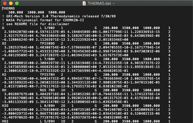
Line 2 - Contains Global temperatures (i.e. 300.000 1000.000 5000.000)

Line 6 - Contains species name (i.e. O) & local temperatures (i.e. 200.000 3500.000 1000.000)

Lines 7-9 - Contain 14 coefficients, 7 each for high & low temperatures, first 7 being high-temperature coefficients.

Similarly, the data (lines 6-9) is repeated for other species.

REASON FOR CHOOSING FILE PARSING:

Engineering problems involve a lot of data and properly maintaining and utilising the data is of at most importance and since the data is available in a .dat file it's easier to extract the data directly,The program shows how effective is it to use MATLAB for parsing the data and use inputs from that data to then pass into functions and get the user defined quantities from the functions.

CODING LOGIC:

After talking the "THERMO.dat" file as input, required data is extracted and unnecessary lines are read and skipped.
First required data are global temperatures which are then stored in individual variables and global temperature range is calculated.
Second, the species name is stored in the array “species”.
Third, local temperature is stored in individual variables,then coefficients are stored in varibles (a1-a14), first seven being the high temperature coefficients and next seven being low temperature coefficients.
Specific heat, Entropy and Enthalpy is calculated with the help of separate functions.
The directory is changed from the default MATLAB directory and all the plots such as specific heat vs temp, entropy vs temp and enthalpy vs temp are saved in folder separate for each species and after saving the directory is changed back to the default MATLAB directory.
Molecular weight of the species is calculated and printed in the command window.
The for loop is repeated 53 times for all the 53 species whose data is present in “THERMO.dat” file and all the plots are saved in their individual folders named with species name.

MATLAB CODE:

clear all
close all
clc

%inputs                                                     %line 5
R = 8.134;

% Loading file
f1 = fopen('THERMO.dat','r');                               %line 9

% Reading the global temperatures                           %line 11
fgetl(f1);
TLINE_1 = fgetl(f1);
A = strsplit(TLINE_1,' ');

for i =1:length(A)
    temp(i) = str2double(A{i});   
end   

global_low_temp = temp(1);
global_mid_temp = temp(2);
global_high_temp = temp(3);

% Temperature Range
T = linspace(global_low_temp,global_high_temp,1000);        %line 25

% skipping lines that are not required                      %line 27
for i=1:3
   fgetl(f1); 
end                                                         %line 30

% Reading the species & their data                          %line 32
for j=1:53
    
TLINE_2 = fgetl(f1);                                        %line 35
B = strsplit(TLINE_2,' ');

% name of the species
species = (B{1});

%local temperatures
low_temp = str2double(B{end-3});  
mid_temp = str2double(B{end-2});
high_temp = str2double(B{end-1});                           %line 44

% reading and converting High temp co-eficients             %line 46
tline_1 = fgetl(f1);
a = strfind(tline_1,'E');

a1 = str2double(tline_1(1:a(1)+3));
a2 = str2double(tline_1(a(1)+4:a(2)+3));
a3 = str2double(tline_1(a(2)+4:a(3)+3));
a4 = str2double(tline_1(a(3)+4:a(4)+3));
a5 = str2double(tline_1(a(4)+4:a(5)+3));

tline_2 = fgetl(f1);
b = strfind(tline_2,'E');

a6 = str2double(tline_2(1:b(1)+3));
a7 = str2double(tline_2(b(1)+4:b(2)+3));                    %line 60

% reading and converting Low temp co-eficients              %line 62
a8 = str2double(tline_2(b(2)+4:b(3)+3));
a9 = str2double(tline_2(b(3)+4:b(4)+3));
a10 = str2double(tline_2(b(4)+4:b(5)+3));

tline_3 = fgetl(f1);
c = strfind(tline_3,'E');

a11 = str2double(tline_3(1:c(1)+3));
a12 = str2double(tline_3(c(1)+4:c(2)+3));
a13 = str2double(tline_3(c(2)+4:c(3)+3));
a14 = str2double(tline_3(c(3)+4:c(4)+3));                   %line 73


% Specific heat                                             %line 76
Cp = specific_heat(a1, a2, a3, a4, a5, a8, a9, a10, a11, a12, T, R, mid_temp);

% Entrophy                                                  %line 79
S = entrophy(a1,a2,a3,a4,a5,a7,a8,a9,a10,a11,a12,a14,T,R,mid_temp);

% Enthalpy                                                  %line 82
H = enthalpy(a1,a2,a3,a4,a5,a6,a8,a9,a10,a11,a12,a13,T,R,mid_temp);

% Plotting
  
% Saving in a folder                                        %line 87
% changing directory
cd('/Users/gulshan/Downloads/skill-lync/Course 1 - Matlab/week 4/report 7  NASA thermo/Species')  
%creating directory
mkdir(species);  
cd(species);                                                %line 92

% Specific heat vs Temperature                              %line 94
figure(1)
plot(T,Cp,'linewidth',3,'color','r')
xlabel('Temperature')
ylabel('Specific heat')
title(sprintf('Specific heat vs Temperature of %s',species));
grid on
saveas(figure(1),'Specific Heat.jpg');                      %line 101

% Entrophy vs temperature                                   %line 103
figure(2)
plot(T,S,'linewidth',3,'color','g')
xlabel('Temperature')
ylabel('Entrophy')
title(sprintf('Entrophy vs Temperature of %s',species));
grid on
saveas(figure(2),'Entropy.jpg');                            %line 110

% Enthalpy vs temperature                                   %line 112
figure(3)
plot(T,H,'linewidth',3,'color','b')
xlabel('Temperature')
ylabel('Enthalpy')
title(sprintf('Enthalpy vs Temperature of %s',species));
grid on
saveas(figure(3),'Enthalpy.jpg');                           %line 119 

%Changing back the directory to Original matlab path        %line 122
cd('/Users/gulshan/Documents/MATLAB') 

%Molecular weight of the species                            %line 124
m_weight = molecular_weight(species);
fprintf('Molecular weight of %s = %f', species, m_weight)
fprintf('n')                                               %line 127

end                                                         %line 129
% End of the program

EXPLANATION:

Lines 5-9

Defining R (Universal gas constant) and loading the “THERMO.dat” file.

Lines 11-25

Reading global temperatures, storing them in individual variables and defining T (Global temperature range).

Lines 27-30

Skipping 3 lines not required from “THERMO.dat”

Lines 32-130

Reading species and their data - Using “for loop” to repeat the same code for all the species.

Lines 35-44

Reading the name of species and saving it in array called “species” and reading local temperatures and storing them in different variables.

Lines 46-60

Since the coefficients are in the form of E^some power, it is easier to find the place of E in the line(explained in coding logic in detail) and using it to separate the coefficients and read the seven high temperature coefficients (a1- a7).

Lines 62-73

Similar logic can be used to read the seven low temperature coefficients (a8-a14).

Line 76-77

Cp (specific heat) is calculated by passing first 5 high temperature(a1-a5), first 5 low temperature coefficients(a8-a12), T(Global temperature range), R(Universal gas constant) and mid_temp (local mid temperature) to function “specific_heat”.

Line 79-80

S (entropy) is calculated by passing first 12 temperature coefficients(a1-a12) and 14^th coefficient(a14), T(Global temperature range), R(Universal gas constant) and mid_temp (local mid temperature) to function “entrophy”.

Line 82-83

H (enthalpy) is calculated by passing first 13 temperature coefficients(a1-a13), T(Global temperature range), R(Universal gas constant) and mid_temp (local mid temperature) to function “enthalpy”.

Lines 87-92

Changing the directory from the default MATLAB directory and creating a folder “species” using “mkdir” command to save Cp, H and S plots for each species in separate folders.

Lines 94-101

Generating Specific heat vs temperature plot and using “saveas” command to save the plot for the particular species whose loop in on.

Lines 103-110

Generating Entropy vs temperature plot and using “saveas” command to save the plot for the particular species whose loop in on.

Lines 112-119

Generating Enthalpy vs temperature plot and using “saveas” command to save the plot for the particular species whose loop in on.

Line 122

Changing back the directory to the default MATLAB directory.

Lines 124-127

Calculating molecular weight for each species and printing them in the command window.

Line 129

End of the for loop, the loop is repeated 53 time i.e. for all the 53 species present in the “THERMO.dat”.

FUNCTIONS:

1. Specific Heat Function

Code:

function Cp = specific_heat(a1, a2, a3, a4, a5, a8, a9, a10, a11, a12, T, R, mid_temp)

  if T <= mid_temp
    Cp = (a1 + a2.*(T) + a3.*(T.^2) + a4.*(T.^3) + a5.*(T.^4)).*R;
    
  else
    Cp = (a8 + a9.*(T) + a10.*(T.^2) + a11.*(T.^3) + a12.*(T.^4)).*R;
  end

end

Formula used:

Explanation:

If local mid temperature is greater than T (Global temperature range) then higher temperature coefficients is used to calculate Cp else low temperature coefficients is used to calculate Cp this is because the local mid temperature lies between Global temperature range.

2. Entropy Function

Code:

function S = entrophy(a1,a2,a3,a4,a5,a7,a8,a9,a10,a11,a12,a14,T,R,mid_temp)

if (T <= mid_temp)
S = R.*(a1.*log(T) + (a2.*T) + ((a3.*(T).^2)/2) + ((a4.*(T).^3)/3) + ((a5.*(T).^4)/4) + a7);

else
S = R.*(a8.*log(T) + (a9.*T) + ((a10.*(T).^2)/2) + ((a11.*(T).^3)/3) + ((a12.*(T).^4)/4) + a14);


end

end

Formula used:

Explanation:

If local mid temperature is greater than T (Global temperature range) then high temperature coefficients is used to calculate Cp else low temperature coefficients is used to calculate Cp this is because the local mid temperature lies between Global temperature range.

3. Enthalpy Function

Code:

function H = enthalpy(a1,a2,a3,a4,a5,a6,a8,a9,a10,a11,a12,a13,T,R,mid_temp)

if (T <= mid_temp)
    
H = R.*T.*(a1 + ((a2.*T)/2) + ((a3.*(T).^2)/3) + ((a4.*(T).^3)/4) + ((a5.*(T).^4)/5) + ((a6./T)));

else
H = R.*T.*(a8 + ((a9.*T)/2) + ((a10.*(T).^2)/3) + ((a11.*(T).^3)/4) + ((a12.*(T).^4)/5) + ((a13./T)));

end

end

Formula used:

Explanation:

4.Molecular weight Function

Code:

function m_weight = molecular_weight(species)

Atoms = {'H','C','N','O','S','Ar'};
Atomic_mass = [1.0078, 12.0107, 14.0067, 15.9990, 32.065, 39.9480];
m_weight = 0;
    for i= 1:length(species)
        for j= 1:length(Atoms)
            if strcmp(species(i),Atoms(j))
                m_weight= m_weight + Atomic_mass(j);
                A= j;
            end
                
        end
            
        B= str2double(species(i));
        if B>1
            m_weight= m_weight + Atomic_mass(A)*(B-1);
        end
    end
end

Explanation:

The program take the array "species" as input and molecular weight is initialised as 0.

Atomic elements and thier atomic mass is defined.

"strcmp" command is used to compare "species" and "Atoms" arrays and using the nested for loop molecular weight is calculated.

When the species contains numercial value such as 2 in O2, species is first converted into matrix and then molecular weight is calculated.

RESULTS:

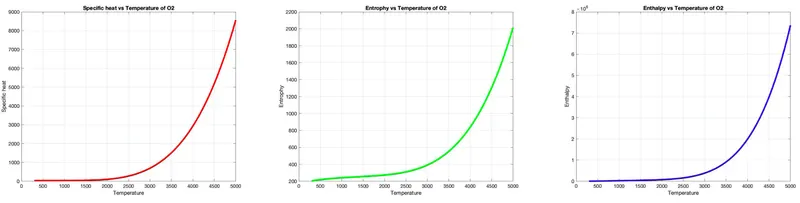
1 . Plots for Oxygen "O2"

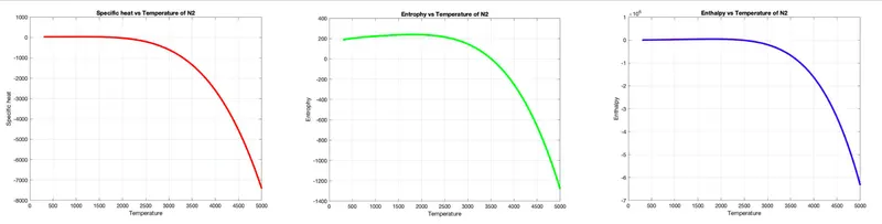
2 . Plots for Dinitrogen "N2"

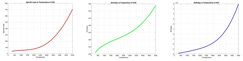
3 . Plots for Carbon dioxide "CO2"

4 . Folder with all the Species with their individual Cp, S and H vs temp plots

(Note - MATLAB is running on macOS 10.15.7 in MACBOOK AIR)

4 . Molecular Mass of Species

CONCLUSION:

SOURCES:

1. Entropy_(classical_thermodynamics)

2. Zemansky, Mark W. (1968). "Chapter 11". Heat and Thermodynamics (5th ed.). New York, NY: McGraw-Hill. p. 275.

3. Open University (2008). S104 Book 3 Energy and Light, p. 59. ISBN 9781848731646.

4. NASA data

Parsing NASA thermodynamic data

Ship work like this
in your own course.

Talk to a career counsellor

Ship work like thisin your own course.

Talk to a career counsellor

Ship work like this
in your own course.