MATLAB code to solve OTTO cycle.

AIM: To write a code to solve OTTO cycle.

GOVERNING EQUATIONS:

For adiabatic process:

PV­­^γ = constant

Where,

P = pressure

V = volume

γ = gamma, heat capacity ratio

Ideal gas law:

P₁V₁/T₁ = P₂V₂/T₂

Volume inside combustion chamber

Thermal efficiency:

N_otto = 1 - 1/r^(γ - 1)

Where r is compression ratio of the engine.

OBJECTIVES:

1 To make PV diagram of the cycle.

2 To calculate Thermal efficiency.

BODY:

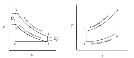
Nicolaus Otto in 1876, proposed a constant volume heat addition cycle which became the basis of present-day spark ignition engines. From the PV diagram, process 0->1 represents the expansion stroke where fuel air mixture is sucked into the combustion chamber through inlet manifold, 1->2 represents the compression of the mixture at the end of compression the pressure of the mixture becomes considerably high and 2->3 represents the combustion, i.e. at this point heat is generated by the combustion of the mixture and the power generated is used to move the piston which in turn moves the crank shaft during 3->4 and 1->0 represents exhaust process.

MATLAB CODE:

%otto cycle
clear all
close all
clc

%inputs
gamma = 1.4; % air
t3 = 2300; % temp. after combustion | k

%State variables
p1 = 1; %bar
t1 = 500; %k

%Engine Geometric parameters
bore = 100; %mm
stroke = 100; %mm
con_rod = 150; %mm
cr = 12;

%calculating the swept volume and the clearance volume
v_swept = (pi/4)*bore^2*stroke;
v_clearance = v_swept/(cr-1);

v1 = v_swept + v_clearance;
v2 = v_clearance;


%state variable at point 2 | after compression
%p1v1^gamma=p2v2^gamma
%p2=p1(v1/v2)^gamma 
p2 = p1*(cr)^gamma;

%p1v1/t1=p2v2/t2 | t2 = p2v2t1/p1v1
t2 = p2*v2*t1/(p1*v1);

constant_c = p1*v1.^gamma;
V_compression = engine_kinematics(bore, stroke, con_rod, cr,180,0);

p_compression = constant_c./V_compression.^gamma;

%state variable at point 3 | after combustion
v3 = v2;
%p3v3/t3=p2v2/t2 | p3 = p2t3/t2
p3 = p2*t3/t2;

constant_c = p3*v3.^gamma;
V_expansion = engine_kinematics(bore, stroke, con_rod, cr,0,180);

p_expansion = constant_c./V_expansion.^gamma;

%state variable at point 4 | after expansion 
v4 = v1;

%p3v3^gamma=p4v4^gamma | p4 = p3(v3/v4)^gamma
p4 = p3*(v3/v4)^gamma;

% pv diagram
figure(1)
hold on

%plotting curve
a1 = plot([v1,v2],[p1,p1],'linewidth',3,'color','b'); M1 = 'suction';
a2 = plot(V_compression,p_compression ,'linewidth',3); M2 = 'compression';
a3 = plot([v2,v3],[p2,p3],'linewidth',3); M3 = 'combustion';
a4 = plot(V_expansion,p_expansion,'linewidth',3); M4 = 'expansion';
a5 = plot([v4,v1],[p4,p1],'linewidth',3,'color','y'); M5 = 'heat rejection';



%plotting points
plot(v1,p1,'*','color','k')
plot(v2,p2,'*','color','k')
plot(v3,p3,'*','color','k')
plot(v4,p4,'*','color','k') 

legend([a1;a2;a3;a4;a5], M1, M2, M3, M4,M5)

title('PV diagram for OTTO cycle')
xlabel('Volume in cc')
ylabel('Pressure in bar')
grid on

%thermal efficiancy 

thermal_efficiancy = (1 - 1/(cr)^(gamma-1))*100;

%end of code

EXPLANATION:

Line numbers are form code image

Lines 6-18

These includes inputs of state variables after expansion i.e. state -1, also engine parameters such as bore, stroke length, compression ratio etc.

Lines 20-25

Swept volume, clearance volume and volume at state-1 i.e. after expansion and state-2 i.e. after compression are calculated.

Lines 28-34

Pressure and temperature at state-2 i.e. after compression is calculated.

Lines 36-39

Engine parameters are passed to the function engine_kinematics and volume at each value of crank angle during compression is calculated and stored in array called V_compression.

V_compression is used to calculate pressure at that point and the values are stored in an array P_compression. These line helps us to determine how volume and pressure changes during combustion.

Lines 41-49

Pressure and volume at state-3 i.e. after combustion is calculated.

Lines 46-49

V_expansion and P_expansion is calculated similarly by passing the engine parameters to the engine_kinematics function. These line helps us to determine how volume and pressure changes during expansion.

Lines 51-55

Pressure and volume at state-4 i.e. after expansion is calculated.

Line 59

Hold on command is used to plot everything in one figure.

Lines 61-66

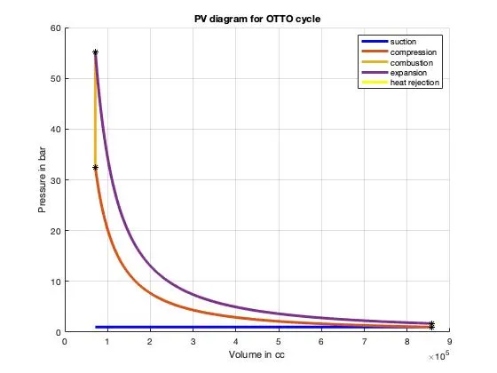
Plot command is used to plot the curves of how pressure and volume changes in otto cycle.

Lines 70-74

Pressure and volume at each point is plotted.

Line 85

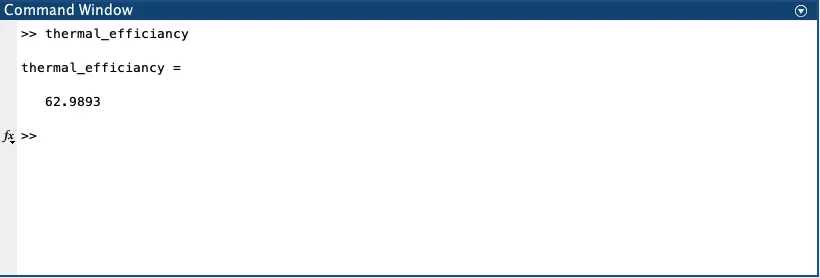
Thermal efficiency is calculated.

FUNCTION CODE:

% this funcition calcualtes how volume changes with crank angle
function [Volume_trace] = engine_kinematics(bore, stroke, con_rod, cr,start_crank, end_crank)

a = stroke/2;
R = con_rod/a;

v_s = pi/4*bore^2*stroke;
v_c = v_s/(cr-1);

theta = linspace(start_crank,end_crank,720);

term1 = 0.5*(cr-1);
term2 = R + 1 - cosd(theta);
term3 = (R^2 - sind(theta).^2).^0.5;

Volume_trace = (1 + term1*(term2-term3)).*v_c;


end
% end of program

EXPLANATION:

The function receives bore, stroke, connecting rod length, starting crank angle and ending crank angle as input.

Lines 13-15

Mathematical formula of how volume inside the chamber varies is broken into three parst for simplicity.

Line 17

Volume trace is calculated and passed to the main code.

RESULT:

Plot - It shows how the volume and pressure during combustion and expansion does not changes linearly.

Thermal efficiency- 62.98%

CONCLUSION:

The study of Otto engine is very much needed as the most used engine i.e. spark engine is based on it and to study the working of the engine its PV diagram is very important. The thermal efficiency is also an important characteristic of the engine.