MATLAB program to solve second order ODEs

AIM: To Solve a 2^nd order differential equation.

GOVERNING EQUATIONS:

d²θ/dt² + (b/m) *dθ/dt + (g/L) *sin(θ) = 0

In the above equation,

g = gravity in m/s²,

L = length of the pendulum in m,

m = mass of the ball in kg,

b=damping coefficient,

θ = angle made by the string w.r.t vertical axis.

OBEJCTIVE:

1. To write a MATLAB program to solve 2^nd order differential equation of a pendulum.
2. To make an animation of the motion followed by the bob of the pendulum.

BODY:

In Engineering, ODE is used to describe the transient behaviour of a system. A simple example is a pendulum.

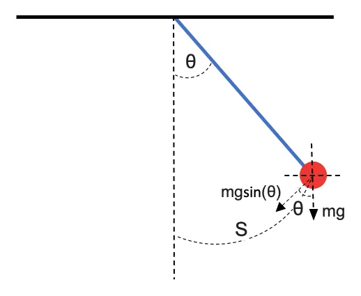
The way the pendulum moves depends on the Newtons second law.

s = L*θ,

v = ds/dt = L*dθ/dt,

a = d²s/dt²= L*d²θ/dt²

F_net = m*a = m* L*d²θ/dt²

F_weight = -m*g*sin(θ)

F_damping = -b* ds/dt = -b* L*dθ/dt

F_net = F_damping + F_weight

m* L*d²θ/dt² = -b* L*dθ/dt + (-m*g*sin(θ))

m* L*d²θ/dt² + b* L*dθ/dt + m*g*sin(θ) = 0

we get a second order Ordinary Differential Equation that describes the position of the "ball" w.r.t time.

d²θ/dt² + (b/m) *dθ/dt + (g/L) *sin(θ) = 0

Converting 2^nd order differential equation into 1^st order differential equation to be solved by ode45.

θ = θ₁

dθ/dt = dθ₁/dt = θ₂

d²θ/dt² = d²θ₁/dt² = dθ₂/dt

Replacing θ₁ and θ₂ in 2^nd order differential equation we get two equations.

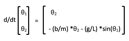
dθ₁/dt = θ₂

dθ₂/dt = - (b/m) *θ₂ - (g/L) *sin(θ₁)

Writing this in matrix form

MATLAB CODE:

%pendulum
clear all
close all
clc

%inputs
b = 0.05; %damping coefficient
g = 9.8; %acceleration due to gravity
l = 1; %length of the string
m = 0.1; %mass of bob

h = [-1,1]; %horizontal axis
v = [-1,0]; %vertical axis

%counter
ct = 1;

%intial conditions
theta_0 = [0,5]; 
x0 = 0;
y0 = 0;

%time 
t_span = linspace(0,20,100);

%solve ode
[t,results] = ode45(@(t,theta) ode_func(t,theta,b,g,l,m), t_span, theta_0);

%plotting
figure(1)
hold on

a1 = plot(t,results(:,1)); M1 = 'displacement';
a2 = plot(t,results(:,2)); M2 = 'velocity';
legend([a1;a2], M1, M2)
grid on
title('Damped pendulum')
xlabel('time')
ylabel('displacement/velocity')

hold off
theta_angle = results(:,1)./l;

for i = 1:length(theta_angle)
   THETA_angle = theta_angle(i);
   x1 = l*sin(THETA_angle);
   y1 = -l*cos(THETA_angle);
   
   figure(2)
   % clears background
   fill([-1.5*l 1.5*l 1.5*l -1.5*l],[-1.5*l -1.5*l 1.5*l 1.5*l],'w');
   
   hold on
   %string
   plot([x1,x0],[y1 y0],'b','linewidth',6)
   %axis
   line = 0*h;
   plot(h,line,'k','linewidth',2)
   g = 0*v;
   plot(g,v,'k--')
   %bob
   plot(x1,y1,'ro','MarkerSize',18,'MarkerFaceColor','r')
   title('Simple pendulum')
   pause(0.3)
   axis([-1.5 1.5 -1.5 1.5])

   P(ct) = getframe(gcf);
   ct = ct+1;  
   
end

% making the video file
movie(P)
videofile = VideoWriter('pendulum_animation.avi','uncompressed AVI');
open(videofile)
writeVideo(videofile,P)
close(videofile)
% end of the program

EXPLANATION:

The lines are from the image of code

Lines 6-13

Contains the inputs from the pendulum like length of the wire, mass of bob etc.

Lines 18-21

Theta_0 array contains initial displacement i.e. zero and initial velocity i.e. five.

And position of the fixed end.

Line 24

t_span contains the interval of time in which the displacement and velocity is required.

Line 27

result is an array in which displacement and velocity are stored.

ode45 is an inbuild MATLAB solver for order differential equations which is based on Runga kutta method.

t, theta, b, g, l and m are passed into a function called ode_func. The results from ode_func along with the t_span and initial values stored in theta_0 is used by ode45 to solve the second order differential equation.

Lines 33-39

First column of the result matrix contains the displacement and the second column contains the velocity of the moving pendulum.

Plot command is used to plot these values against time and hold on command is used to plot them on the same plot.

Line 42

Calculates the angle made by the string w.r.t to vertical axis at particular displacement and stored in an array theta_angle.

Lines 44-47

For loop is used to get individual values from theta_angle array and store them in THETA_angle and with the help of this the position of moving end points are calculated.

Line 55

With the help of coordinates of both the end points of the string, the string is plotted.

Lines 57-60

It is used to make the axis

Lines 61-65

This is used to plot the bob.

Lines 73-77

This is used to make the video file from the already saved frames, saved in the array P using getframe command.

FUNCTION:

function [dtheta_dt] = ode_func(t,theta,b,g,l,m)

theta1 = theta(1);
theta2 = theta(2);
dtheta1_dt = theta2;
dtheta2_dt = -(b/m)*theta2 - (g/l)*sin(theta1);
dtheta_dt = [dtheta1_dt; dtheta2_dt];

end

EXPLANATION:

dtheta_dt matrix contains two variables dtheta1_dt and dtheta2_dt which is used to solve for displacement and velocity.

ERROR/EXPLANATION:

Passed less arguments in the ode_func, overcome the error by passing correct numbers of arguments.

RESULT:

1. Graph between displacement & velocity vs time.

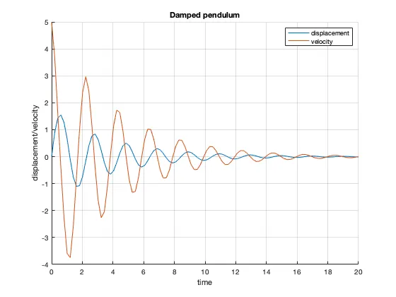
As we can see the bob was at the mean position(s=0 m) at the start and an initial velocity of 5m/s2 was given and as time progress the bob's velocity and displacement limits to zero.

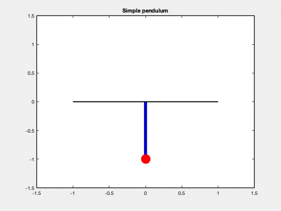
2 . Animation of the motion of pendulum

CONCLUSION:

Different order differential equations are very common in engineering and solving these equations to get different parameters are very important.

There are various solvers based on various numerical methods to solve these equations, ode45 being one of them which is based on 4^th order Ranga kutta method. Hence by solving the odes we can simulate how the values change w.r.t to change in parameters and can choose the optimum value of parameter for the process required.