Week 4 - Genetic Algorithm
Aim : Optimise the stalagmite function and find the global maxima of the function in MATLAB.
Objective :
1.Write a code in MATLAB for evaluation of stalagmite function.
2.To understand the concept of genetic algorithm and use inbuilt ga function to optimise the stalagmite function.
3.Find global maxima and try ways to minimise the uncertainty.
Theory:
1.Genetic Algorithm.
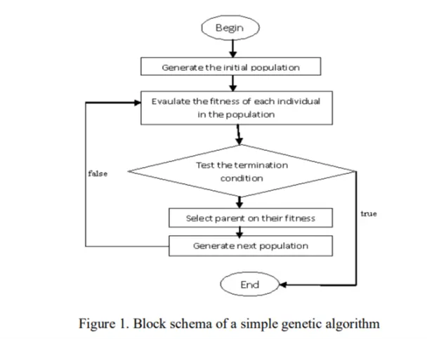
A genetic algorithm applies the biological principles of natural evolution in the artificial systems relying on biologically inspired operators such as selection,cross over and mutation.
GA generates a population to start with in a totally random manner. Certainly, the initial general fitness of these individuals is very bad.
The individuals are evolved in the next iterations which are called generations. In each generation, the individuals are assessed according to the fitness they have. The individuals that are selected(parents) to create new individuals offspring are selected based on their fitness – the more adequate they are, the more the chances they have for reproduction.
Afterwards, the population of the next generation is created through the genetic operators. This procedure continues until the termination criterion of the genetic algorithm is met.
2.Genetic Operators.
Crossover
The main feature of GA is the use of crossover. Crossover, also called recombination, is an operator that creates new individuals from current population, combining pieces of information coming from different individuals of the population.
Mutation
Mutation is a very easy method to create a new individual. This method can be used after the crossover method. Mutation does a very simple thing: it replaces one or more genes randomly selected in the individual’s representation.
3.ga solver.
ga() solver in MATLAB is pre defined,inspired by natural selection process and it works on genetic algorithm theory to find minimum of the function.ga is used for optimization purpose to get high quality results.
4.Syntax.
x = ga(fun,nvars) : finds a local unconstrained minimum x .nvars = number of variables
x = ga(fun,nvars,A,b) finds a local minimum. Subject to the linear inequalities A*x ≤ b.x is transposed
x = ga(fun,nvars,A,b,Aeq,beq) finds a local minimum x to fun, subject to the linear equalities Aeq*x = beq and A*x ≤ b.
x = ga(fun,nvars,A,b,Aeq,beq,lb,ub) defines a set of lower and upper bounds.
x = ga(fun,nvars,A,b,Aeq,beq,lb,ub,nonlcon) The function returns vectors C and Ceq, representing the nonlinear inequalities and equalities respectively.
x = ga(fun,nvars,A,b,[],[],lb,ub,nonlcon,IntCon) requires that the variables listed in IntCon take integer values.
x = ga(fun,nvars,A,b,Aeq,beq,lb,ub,nonlcon,options) minimizes with optimization parameters replaced by values in options.Create options using optimoptions.
5.Termination Criteria.
The genetic algorithm passes from one generation to the other until the termination criteria of the algorithm is met.
A solution is found that satisfies minimum criteria
The most used criteria for the termination of the algorithm is a fixed maximal number of generations.
There is another strategy uses the criteria of the population’s convergence, GA pushes the major part of the population to converge in one single solution. So, when the sum of deviations between individuals becomes smaller than a predefined value, the algorithm can terminate.
Also the algorithm may terminate as result of the improvement of the best solution after a certain number of generations.
Also, different strategies can be combined together for terminating a genetic algorithm.
6.Significance of running more iterations.
Now we know the working of the ga solver.More the iterations better high quality results will it produce.With more iterations more generations will be created which will help to converge the final reuslt.The randomness decrease as we increase the population size.To see this effect in action kindly see the case 3 code and compare case 3 results with case 1 results.
Formulae:
`f=fx1*fx2*fy1*fy2` is the stalagmite function whose global maxima has to be evaluated.
where;
`fx1=sin((5.1*pi*x)+0.5)^6`
`fy1=sin((5.1*pi*y)+0.5)^6`
`fx2=exp(-4*log(2)*(x-0.0667)^2/0.64)`
`fy2=exp(-4*log(2)*(y-0.0667)^2/0.64)`
Main code :
clear all
close all
clc

%defining search space
x=linspace(0,0.6,150);
y=linspace(0,0.6,150);

%setting number of ga iterations
num_cases=50;

%creating 2D grid and evaluating stalagmite function
f=get_stalagmite(x,y);


%Case 1 : Statistical Behaviour
tic
for i=1:num_cases
    [inputs,f_opt(i)]=ga(@stalagmite,2);
    x_opt(i)=inputs(1);
    y_opt(i)=inputs(2);
end
studytime_1=toc;        %timer to measure time required for loop completion

figure(1)
subplot(2,1,1)          %plotting in first row
hold on
surfc(x,y,-f)
shading interp
plot3(x_opt,y_opt,-f_opt,'marker','o','markersize',5,'markerfacecolor','r')
title('unbounded inputs')
xlabel('x optimum')
ylabel('y optimum')
zlabel('f optimum')

subplot(2,1,2)          %plotting in second row
plot(-f_opt)
xlabel('iterations')
ylabel('function maximum')


%Case 2 : Statistical Behaviour with Upper & Lower Bounds
tic
for i=1:num_cases
    [inputs,f_opt(i)]=ga(@stalagmite,2,[],[],[],[],[0;0],[1;1]);
    x_opt(i)=inputs(1);
    y_opt(i)=inputs(2);
end
studytime_2=toc;

figure(2)
subplot(2,1,1)          %plotting in first row
hold on
surfc(x,y,-f)
shading interp
plot3(x_opt,y_opt,-f_opt,'marker','o','markersize',5,'markerfacecolor','r')
title('bounded inputs')
xlabel('x optimum')
ylabel('y optimum')
zlabel('f optimum')

subplot(2,1,2)          %plotting in second row
plot(-f_opt)
xlabel('iterations')
ylabel('function maximum')


%Case 3 : Increasing number of ga iterations
options=optimoptions('ga','populationsize',170);

tic
for i=1:num_cases
    [inputs,f_opt(i)]=ga(@stalagmite,2,[],[],[],[],[0;0],[0.2;0.2],[],[],options);
    x_opt(i)=inputs(1);
    y_opt(i)=inputs(2);
end
studytime_3=toc;

figure(3)
subplot(2,1,1)          %plotting in first row
hold on
surfc(x,y,-f)
shading interp
plot3(x_opt,y_opt,-f_opt,'marker','o','markersize',5,'markerfacecolor','r')
title('bounded inputs with modified population')
xlabel('x optimum')
ylabel('y optimum')
zlabel('f optimum')

subplot(2,1,2)          %plotting in second row
plot(-f_opt)
xlabel('iterations')
ylabel('function maximum')
Code explaination :
All a good measure of coding we start this code as well by using clear all, close all and clc.We define our search space by using linspace() command for x and y variable.We need to decide the number of iterations for ga function.Here we set the value as 50.
We call the get_stalagmite() function for evaluating the given function in the search space defined by us.
We have splitted the entire main code in three seperate cases.Lets take a look at the case 1 code.We make use of the ga solver for optimization by passing two variables and getting the maximum values as output.The function returns two optimum value of the function (in our case the maximum value) and also show the x and y value at which this maximum value occurs.We carry this iteration 50 times as decided earlier.To measure how much time it took to complete 50 iterations we use tic and toc.For better understanding of the results we are plotting two graphs in one figure hence we make use of subplot() function.In the first row of the figure we plot the surface of stalagmite function.And in the same graph we mark the maximum points i.e. f optimum.Since this is a 3D plot we use plot3().The last step in case 1 is to plot the f optimum obtained from ga iterations.But since we have modified the code for maxima condition we plot negative value of f optimum.
Moving on to the case 2.As seen from the result of first case we can observe that the maximum value obtained is not the global maxima but we get many local maxima.Global maxima is one of those and all these points are all over the place because ga doesnt know the bounds within which it has to work.For this reason we mention the upper and lower bounds in the ga solver(ga(@stalagmite,2,[],[],[],[],[0;0],[1;1]).This is the only difference between case 1 and 2.We calculate the time elapsed and plot the results similarly as mentioned in the previous case.This optmizes the function hugely.
As seen that limiting the ga solver in bounds we can achieve better consistent results we narrow down our bounds.And to find the global maxima we increase the initial population size to 200 (by deafult in our case the population size 50).This is done with the help of optimoptions().Higher the population size slower the code gets but this trade off is viable as we are able to get the global maxima.We calculate the time elapsed and plot the results similarly as mentioned in the previous case.
Function 1(get_satalagmite) Code :
%creating a two dimensional grid
function f=get_stalagmite(x,y)

[xx, yy]=meshgrid(x,y);

    for i=1:length(xx)
         for j=1:length(yy)
             input_vector(1)=xx(i,j);
             input_vector(2)=yy(i,j);
             f(i,j)=stalagmite(input_vector);
         end
    end
end
Code explaination :
We have provided the range of x and y in the main program. Our aim is to plot a surface for which we need a 2D array which is created using meshgrid().After that we need to send 2 variables to the stalagmite function for evaluation.This is done by using two for loop in conjunction and we get the output 'f' by calling the stalagmite function.
Function 2(stalagmite) Code :
%evaluating stalagmite function
function f=stalagmite(input_vector)

x=input_vector(1);
y=input_vector(2);

fx_1=(sin((5.1*pi*x)+0.5)).^6;
fy_1=(sin((5.1*pi*y)+0.5)).^6;

fx_2=exp(-4*log(2)*(x-0.0667)^2/0.64);
fy_2=exp(-4*log(2)*(y-0.0667)^2/0.64);

f=-(fx_1*fx_2*fy_1*fy_2);

end
Code explaination :
This code is to written to evaluate the stalagmite function.We pass in input as input_vector which has 2 values(x,y) in it. We assign the values and then simply calculate all the four terms by using the formulae mentioned in the earlier part.This function will give output f which is multiplication of all the four terms.But since we need to find maxima we return the oput function as a negative value.
Results:
Case 1.
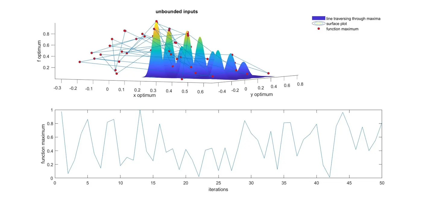
It can be seen that the ga solver is finding the local maxima of the function.And because there are no bounds the results are randomised all over the place.It can also be visualised much clearly from the second subplot that the the value of f optimum varies way too much.
Case 2.
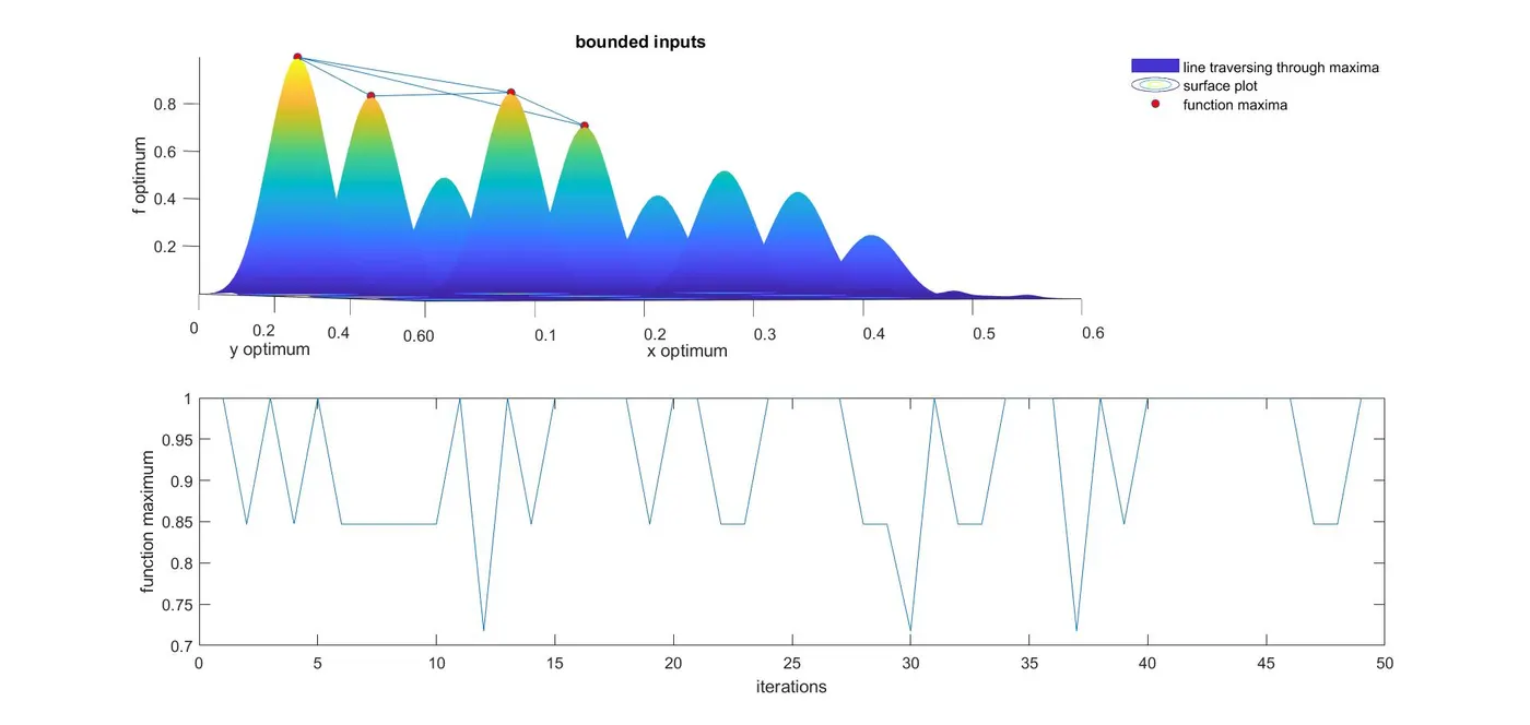
When we bound our searchspace,the ga solver is able to work more precisely.Even though we did not find the globa maxima our results were confined to four points.
Case 3.
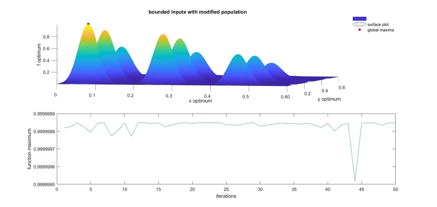
When we lower the boundary constraint even more and also increase the population size ga solver was able to predict the global maxima.And this results in having consistent output value.All the f optimum values lie very close to 1 as seen in the second sub plot.
Conclusion :
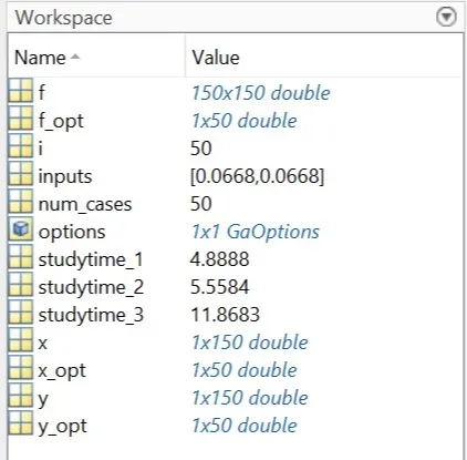
The above attached image is the workspace.We can see the runtime for all the three cases.This shows that higher the population size slower the ga program gets but in return we do get consistent results.
In our case the global maxima was almost 1 and it was found at 0.0668,0.0668.
Error Faced :
This error was faced because xx,yy are present in seperate function and that function gives output as 'f' not xx,yy
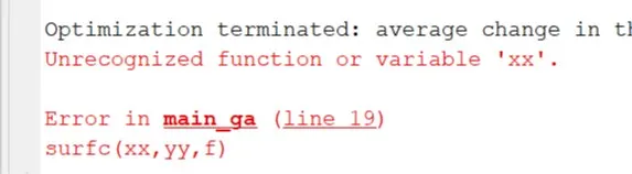
The error was solved by changing the code to surfc(x,y,f).
Refernces :
What is Genetic Algorithm in MATLAB
https://www.youtube.com/watch?v=1i8muvzZkPw
ga solver in MATLAB Documentation
https://in.mathworks.com/help/gads/ga.html
Mathworks Q & A section
https://in.mathworks.com/matlabcentral/answers/52240-how-to-find-max-fuction-with-genetic-algorithm
Wikipedia
https://en.wikipedia.org/wiki/Genetic_algorithm