Week 3 - Solving second order ODEs

Aim:To simulate the behavior of a simple pendulum motion using MATLAB.

Objective:

1.To write a program to solves the ODE that represents the equation of motion of a simple pendulum with damping.

2.To compute results and plot graphs.

3.Create a small video to animate the motion of the simple pendulum.

Formula:

The following formula represents motion of simple pendulum with damping

`(d^2theta)/dt^2+(b/m)(d theta)/dt+(g/l)sin theta=0`

Theory:

An ideal simple pendullum is mass attached to a weightless string hunged at a frictionless support.But realistically the support cannot be frictionless and niether the string can be weightless and also the real pendulum is subjected to air drag.If the pendullum is given a swing the pendulum carries out Simple Harmonic Motion and the pendulum will eventually come to rest.To stop the pendulum much quickly damper can be used.The below mentioned second order ODE represents the motion.

`(d^2theta)/dt^2+(b/m)(d theta)/dt+(g/l)sin theta=0`

We can solve ODE's in MATLAB using ODE solvers.The most common is ode45.But to use this solver we need to convert the second order ODE into two first order ODE.

Let,

`theta=theta 1`

`(d theta)/(dt)=(d theta 1)/dt=theta 2`                     ...Equation 1

`(d^2 theta)/(dt^2)=(d^2 theta 1)/(dt^2)=(d theta 2)/dt`          ...Equation 2

Substituting the values of both equations in the second order ODE;we get

`(d theta 2)/dt+(b/m)theta 2+(g/l)sin theta 1=0`

Rearranging;

`(d theta 2)/dt =-(b/m)theta 2-(g/l)sin theta 1`          ...Equation 3

We will using these equations further to create a function.

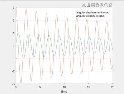
In our case the mass of bob is 1kg with the pendulum being 1m long.The damping coefficient is given b=0.05.We have to compute the motion of pendulum for a time period of 20 seconds.The initial conditons are given to be : angular displacement=0 rad,angular velocity=3 rad/sec.

Main Program Code:

%Pendulum motion using 2nd order ODE
clear all
close all
clc

%inputs given
l=1;                                                         %length of pendulum in m
m=1;                                                         %mass of bob in kg
b=0.05;                                                      %damping coefficient
g=9.81;                                                      %acc. due to gravity in m/s^2
theta_0=[0;3];                                               %initial conditions 
time_span=linspace(0,20,500);                                %time 

%using ode45 solver
[t,results]=ode45(@(t,theta) ode_func(t,theta,b,g,l,m),time_span,theta_0);

%plotting result
figure(1)
hold on
plot(t,results(:,1),'linewidth',2)                           %plotting ang. disp vs time
plot(t,results(:,2),'linewidth',2)                           %plotting ang. vel vs time
xlabel('time')
grid on
legend('angular displacement in rad','angular velocity in rad/s')

ct=1;                                                         %counter
for i=1:length(results(:,1))
    
    %fixing top end of pendulum
    x0=0;
    y0=0; 
    
    %evaluating coordinates of bob
    x1=l*sin(results(i,1));
    y1=-l*cos(results(i,1));
    
    %plotting pendulum motion
    figure(2)
    plot([-1 1],[0 0],'color','g','linewidth',2)               %support bar for pendulum
    plot(x0,y0,'o','markerfacecolor','r')                      %point where pendulum in tied  
    hold on
    plot([x0 x1],[y0 y1],'color','b','linewidth',2)            %creating pendulum rod
    plot(x1,y1,'o','markersize',20,'markerfacecolor','r')      %plotting bob
    axis([-1.25 1.25 -1.25 0.5])
    grid on 
    xlabel('x axis')
    ylabel('y axis')
    hold off
    pause(0.005)
    
    A(ct)=getframe(gcf);                                      %capturing frame for animation
    ct=ct+1;                                         
    
end

%creating animation 
movie(A)
videofile=VideoWriter('pendulum.avi','Uncompressed AVI');
open(videofile)
writeVideo(videofile,A)
close(videofile)
    
    

Code Explaination: 

We will simply start the code by assigning all the inputs given in the problem statement.i.e. b,g,l,m.We are also provided with the initial conditions of bob at time=0 i.e. displacement is 0 rad and angular velocity is 3 r/s. We are asked to calculate the motion for a time span from 0 to 20sec.We create that time span with 500 intervals using linspace() command.

We use the ode45 solver next.whose syntax follows as ode45(@(input parameters) our_defined_function,integral limits,intial conditions).The solution acquired is stored in results matrix.

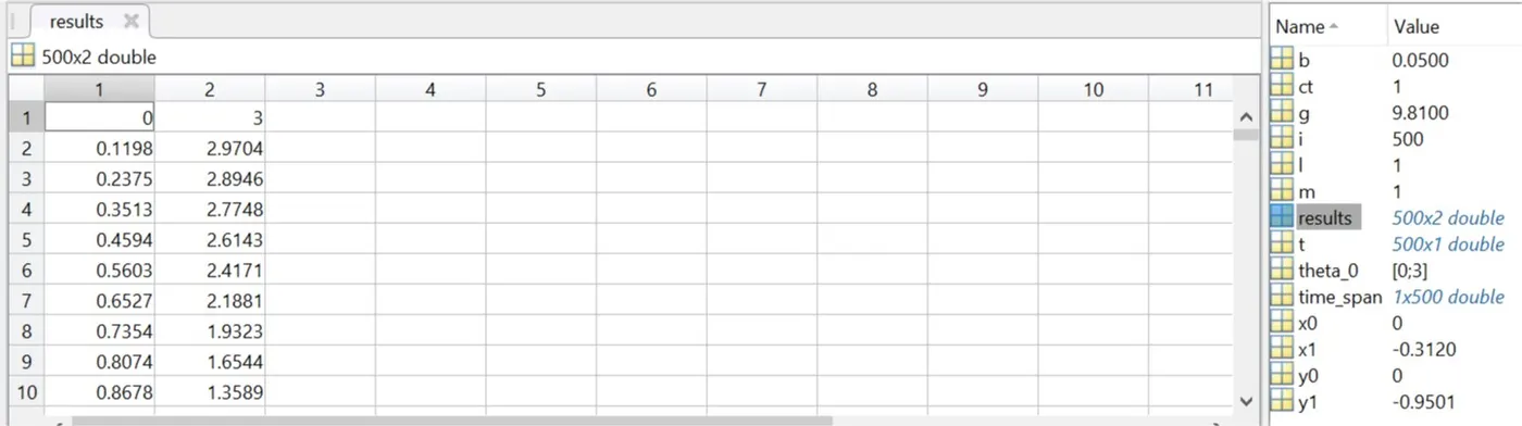
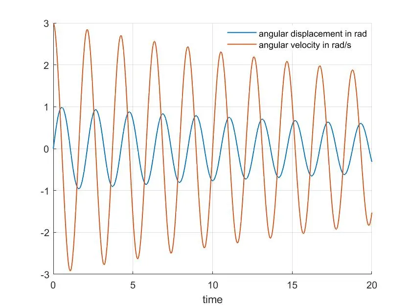
The first column of results matrix is angular displacement and the second column is angular velocity.Since we have the displacement and velocity , we  plot the graph of both with respect to time using plot function.

Our requirement is to plot the motion of the pendulum.For the we make use of for loop which iterates from 1 till the length of results table.First we fix the top end of the pendulum at the origin.Then we calculate the coordinates of other end by using simple trignometry.(Note:Values are already in radians so do not use sind()).We shall plot the pendulum in three stages using plot() command.First we plot the support bar and highlight the support point os suspension.Secondly we join the calculated points to origin to get the rod of pendulum.And lastly we create the bob at the end of the rod.Make sure to use hold on and hold off to display everything required in the plot.

Now we can see the animation at this stage but we need to capture this.For this we are required to create a counter variable previous to our for loop and increase its value for every loop.We capture one frame for each for loop executed by usung the getframe() command and store it in 'A'.We create a video using the movie() command and mention the name and format of the videofile.To finalize  we open the videofile , write the videofile created and to terminate we close the file. 

Function Code:

function [dtheta_dt]=ode_func(t,theta,b,g,l,m)

theta1=theta(1);
theta2=theta(2);

dtheta1_dt=theta2;
dtheta2_dt=-(b/m)*theta2-(g/l)*sin(theta1);

dtheta_dt=[dtheta1_dt;dtheta2_dt];
end

Code Explaination:

We create a function named ode_func. It represents this system of equations as a function that accepts input arguments: t,theta,b,g,l,m .The entire function code is simply conversion of mathematical equation 1,2 and 3 derived earlier to MATLAB code.We represent theose equations in matrix form.

Results:

1.We get two columns in the results table.The first column represents the angular displacement for the time span of 20 seconds with 500 intervals in between those 20 seconds.In the similar way the second column represents the angular velocity.We can see this in the image attached below:

2.Now we have all the required values we can plot the graph for angular displacement vs time and angular velocity vs time both in the same graph.

3.Finally the animation of the motion of the simple pendulum is shown in the below video.To access the video file kindly use the youtube link :

https://www.youtube.com/watch?v=bT84ryrHuwY

Erros Faced and Rectification :

No command oriented errors were present but rather graphical errors were present.

1.The first problem  I had was that the pendulum graph was plotted inverted.

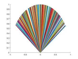
The solution to this was quite easy. Only had to add '-' sign when calculating the y1 co ordinate.

2.The second error faced was that the we need to see only one instance of the pendulum rather than all the positions.

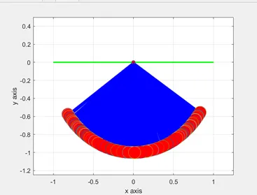
The solution was to specify the hold off command before exiting the loop.

3.The final error was that the legends were not being displayed

This is an AMD graphics driver issue which can be rectified by simply mentioning the linewidth of over 0.5 as 0.5 is the default value.