Air standard cycle : Otto cycle

Aim: To evaluate efficiency of an engine using otto cycle and calculating its efficiency.

Objective: Evaluating all the parameters of engine. Plotting P-V diagram for otto cycle and calculating thermal efficiency of the engine.

Body:

Otto cycle is a thermodynamic cycle used for spark ignition engines.An ideal otto cycle consists of four processes.It starts with isentropic compression of the gas.A spark is ignited and constant volume combustion takes place.Once the gas is burnt it expands isentropically in the engine pushing the piston down.The heat is rejected in the next constant volume process.And the cycle repeats.

For our analysis we are having an engine whose bore diameter is 0.1m,having stroke length of 0.1m.The compression ratio of our engine is 6 and the connecting rod length is 0.15m.It is given that the ratio of specific heats `gamma`is 1.4.The maximum working temperature of our engine is 1500K and the engine starting temperature is 400K.

Formulae:

Besides from these given inputs all the other remaining parameters can be evaluated by using the formulae

PV = nRT This can be rewritten as `PV/T=C` where C is constant.

We will discuss during the code explaination how all the parameters are calculated by manipulating the above formulae for various processes.

Code 1:

%otto cycle

close all
clear all
clc

%inputs
d=0.1;%bore diamenter
l=0.1;%stroke length
r=6;%compression ratio
conrod=0.15;%connecting rod length
gamma=1.4;%ratio of sp. heats

%engine parameters at point 1
p1=101325;
t1=400;
vs=(pi/4)*d^2*l;%swept volume
vc=vs/(r-1);%clearance volume
v1=vs+vc;

%engijne parameters at point 2
%process 1-2 isentropic compression
v2=vc;
p2=p1*(v1/v2)^gamma;
t2=t1*((p2*v2)/(p1*v1));

%compression stroke
V_compression=engine_kinematics(d,l,r,conrod,180,0);
c=p1*v1^gamma;%c is constant
P_compression=c./(V_compression).^gamma;

%engine parameters at point 3
%process 2-3 constant volume combustion
v3=v2;
t3=1500;
p3=p2*(t3/t2);


%engine parameters at point 4
%process 3-4 isentropic expansion
v4=v1;
p4=p3*(v3/v4)^gamma;
t4=t1*(p4/p1);

%expansion stroke
V_expansion=engine_kinematics(d,l,r,conrod,0,180);
c=p3*v3^gamma;%c is constant
P_expansion=c./(V_expansion).^gamma;


%thermal efficiency
%efficiency=1-(1/r^gamma-1)
thermal_efficiency=1-(1/r^0.4);

%plotting 

%volume variation during isentropic processes
figure(1)
vol_trace=engine_kinematics(d,l,r,conrod,0,360);
plot(vol_trace)

%plotting P-V diagram for otto cycle
figure(2)
hold on
plot(V_compression,P_compression,'color','b')
plot(V_expansion,P_expansion,'color','b')
plot([v2 v3],[p2 p3],'-*','markersize',3,'markeredgecolor','r','color','b')
plot([v4 v1],[p4 p1],'-*','markersize',3,'markeredgecolor','r','color','b')
xlabel('volume')
ylabel('pressure')

%plotting thermal effi vs compression ratio
figure(3)
eff_otto(1.3,1.4,1.67);

Code Explaination 1:

We input the given values d,r,l,conrod and gamma. From these given values we calcualte swept volume `vs=(pi/4)*d^2*l` and clearance volume `vc=(vs)/(r-1)`.We have p1 and t1 given now we can calculate v1(`v1=vs+vc`).For calculating parameters at point 2 , we know v2 so to calculate p2 we use the relation `p1v1^gamma=p2v2^gamma`.Similarly t2 can be calculated using `(p1v1)/(t1)=(p2v2)/(t2)`.The volume along the isentropic compression is calculated by calling the function engine_kinematics.As we mentioned earlier `pv^gamma=constant`we can calculate the pressure along the compression curve. Process 2-3 is constant volume heat addition therfore v3=v2 and we also know the temperature at point 3 the remaining pressure p3 can be calculated by using `p3=p2*((t3)/(t2))`.The next process is isentropic expansion and the volume along this curve can be calculated by again calling the engine_kinematic function by simply changing the start_crank angle and end_crank angle. And the last process is constant volume heat rejection.v4 and v1 are same therefore the remaining pressure p4 can be calculated using `p4=p3*((v3)/(v4))^gamma` and temperature t4 by using `t4=t1*((p4)/(p1))`.Finally we calculate the thermal efficiency of the system by using `eta=1-1/r^(gamma-1)`. After computing all the parameters we move on towards plotting the required results, which we would discuss in the results parts of this article.

Code 2:

%volume variation  during isentropic process in otto cycle

function [V]= engine_kinematics(d,l,r,conrod,start_crank,end_crank)

a=l/2;
R=conrod/a;

theta=linspace(start_crank,end_crank,100);

vs=(pi/4)*d^2*l;%swept volume
vc=vs/(r-1);%clearance volume

%volume variation formula
%V/vs = 1+0.5(r-1)[R+1-cos(theta)-(R^2-sin(theta)^2)^0.5]
term1=0.5*(r-1);
term2=R+1-cosd(theta);
term3=(R^2-sind(theta).^2).^0.5;

V=(1+term1*(term2-term3)).*vc;
end

Code Explaination 2: Function engine_kinematics

The above code is of the function used to calculate and trace volume for isentropic process.The volume does not change linearly but it varies according to the formulae `V/v = 1+0.5(r-1)[R+1-cos(theta)-(R^2-sin(theta)^2)^0.5]`.In this function we are providing bore diameter,stroke length , compression ratio ,connecting rod length, engine start crank angle and engine stop crank angle as inputs. Since the formula is too big and might confuse while coding we brreak the code in three different parts term1 term2 and term3. We calculate swept volume , clearance volume and finally input all the values in equation and get 100 values of volume.We will use these values in the main program to calculate the values of volume during compression stroke and expansion stroke. These values of volume are then used to calculate values of pressure during compression and expansion stroke.

Code 3:

%efficiency curve for otto cycle
function efficiency=eff_otto(gamma1,gamma2,gamma3)

r=linspace(1,12,50);

eff1=1-(1./r.^(gamma1-1));
eff2=1-(1./r.^(gamma2-1));
eff3=1-(1./r.^(gamma3-1));

hold on
plot(r,eff1,'color','r')
plot(r,eff2,'color','g')
plot(r,eff3,'color','b')
xlabel('compression ratio')
ylabel('thermal efficienct')
end

Code Explaination 3: Function eff_otto

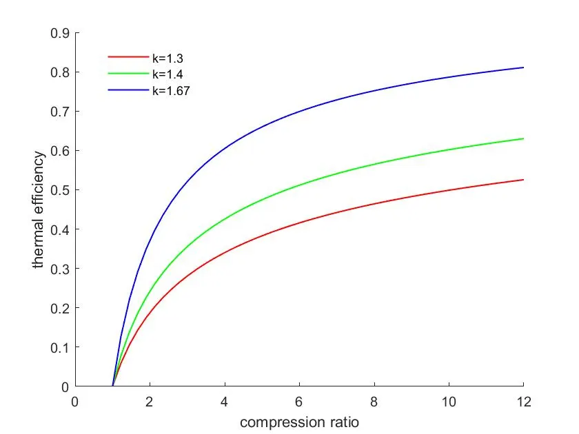
The above code is used to show the variation between efficiency of otto cycle and compression ratio as per the formula for thermal efficiency `eta=1-1/r^(gamma-1)`.

As seen from the formula it is evident that higher the compression ratio higher would be the thermal efficiency.But if we increase the compression ratio way too much than we may face the issue of Detonation. Hence, for spark ignition engines the compression ratio is kept between 6 and 12 .

The second way to improve the efficiency is by varying the ratio of specific heats `gamma`.We can see the variation for three values of `gamma`

In our code we will range the value of compression ratio using linspace command.We can see the variaton for three values of `gamma` and plot the thermal efficiency for each case.

We call this function in our main program and input three values of `gamma`.As seen in the code eff1 is the thermal efficiency for `gamma`=1.3 ,eff2 for `gamma`=1.4 and eff3 for `gamma`=1.67.The curves for each of the following is displayed in red green and blue colour respectively.

Results:

To get the results we plot three different graphs using the plot command.

Figure 1: We plot the volume variation againt theta.This figure doesnt show the trace of our problem but lets us see how the volume varies during the complete otto cycle.For demonstration purpose our `theta`varies between `0^o` and `360^o`

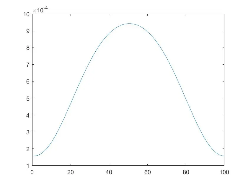
Figure 2:This is the desired PV diagram for otto cycle.We plotted 4 different process and connected all of these to display the complete cycle.All the four points are displayed in red astericks.

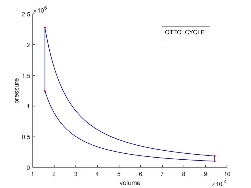
Figure 3:The last figure show the varaition between thermal efficiency and compression ration.The compression ratio varies from 1 to 12 and we plot three differnt curves for three different values of `gamma`.