Week 4 - Genetic Algorithm

Genetic algorithm

Objective:

To write a code in Matlab to optimize the stalagmite function and find the global maxima of the function and to plot graphs for all three studies.

Introduction:

A genetic algorithm is a search experiential that is stimulated by Charles Darwin’s theory of natural evolution. The genetic algorithm is a method for solving both constrained and unconstrained optimization problems that are based on natural selection, the process that drives biological evolution. At each step, the genetic algorithm selects individuals at random from the current population to be parents and uses them to reproduce the next generation. Over successive generations, the population evolves towards an optimal solution.

Phases in the genetic algorithm:

1. Initialization of population(coding)

the code generates its random population of defined size and from that population, the code evaluates the fitness of the members of the population according to which it forms a new population-based on no. of iterations performed.

2. Fitness function

It is that function which we have to optimize and its optimization is done with the help of the number of generations which have been formed by the code in accordance with the fitness value of each member-generated, these fitness values are used for the reproduction of the children.

3. Selection

The idea of the selection phase is to select the fittest individuals and let them pass their genes to the next generation. The main goal of this phase is to find the region where the chances of getting the best solution are more.

• The genetic algorithm uses three main types of rules at each step to create the next generation from the current population, they are

Selection rule: selects the individuals, called parents that contribute to the population at the next generation.

Crossover rule: combine two parents to form children for the next generation.

Mutation rules: apply random changes to individual parents to form children.

Syntax of ga

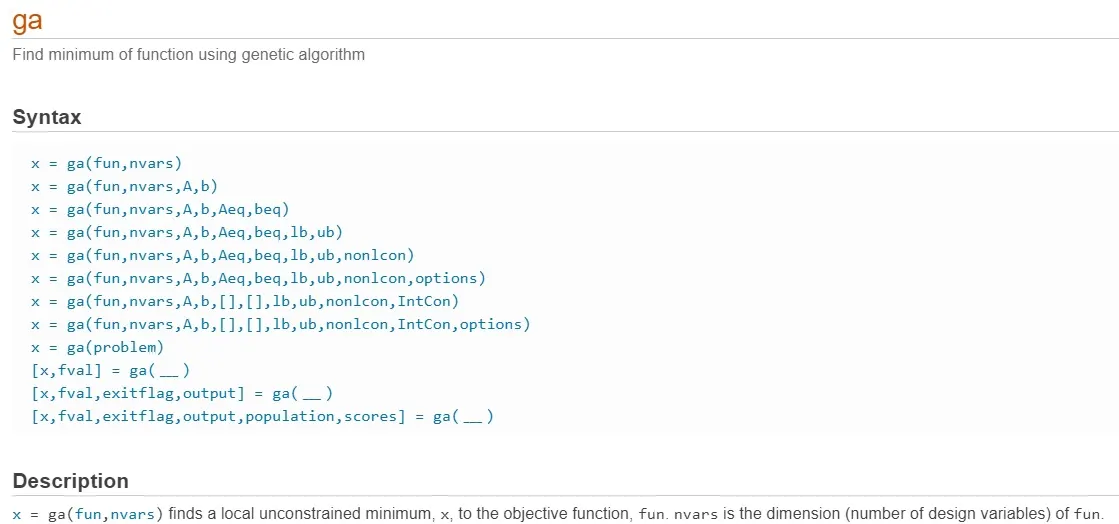
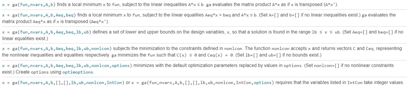
x : optimum solution

fun : fitness function

nvars : number of variables

A,b :linear inequality constraints

Aeq,beq : linear equality constraints

lb : lower bound(limit)

ub : upper bound(limit)

options : to set population size to minimize with non-default options

IntCon : to get a solution in an integer

nonIcon : use for nonlinear constraints

exitflag : reason ga stopped

output : information about the optimization process

population : final population

scores : final scores

Stalagmite function:

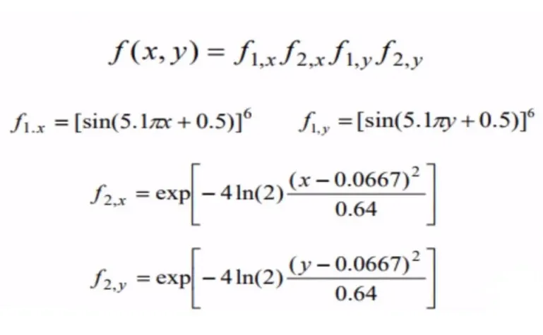
Matlab function code for the stalagmite:

The Matlab file of the stalagmite function code has been uploaded to google drive and the access link to the file is

https://drive.google.com/file/d/10Fy7_6dx-1p6ugJ5xeoStFhNTGxvkGat/view?usp=sharing

function[f] = stalagmite(input_vector)

x = input_vector(1);
y = input_vector(2);

f1_x = (sin(5.1*pi*x+0.5)).^6;
f1_y = (sin(5.1*pi*y+0.5)).^6;
f2_x = exp((-4*log(2))*((x-0.0667).^2)./0.64);
f2_y = exp((-4*log(2))*((y-0.0667).^2)./0.64);

f = -(f1_x.*f1_y.*f2_x.*f2_y);
end

Matlab code for the optimization of the stalagmite function and to find the global maxima:

The Matlab file of the optimization of the stalagmite function has been uploaded to google drive and the access link to the file is https://drive.google.com/file/d/1pqSSOnxo9Y8VVv6qZDFMQcQH-Zbtwuek/view?usp=sharing

clear all
close all
clc

%Defining search space
x = linspace(0,0.6,150);
y = linspace(0,0.6,150);

%Creating a 2Dimensional mesh
[xx yy] = meshgrid(x,y);

%Evaluating the stalagmite function
for i = 1:length(xx)
    for j = 1:length(yy)
        input_vector(1) = xx(i,j);
        input_vector(2) = yy(i,j);
        f(i,j) = stalagmite(input_vector);
    end
end
surfc(xx,yy,-f)
xlabel('x value')
ylabel('y value')
shading interp
[inputs,fval] = ga(@stalagmite,2);



%Study 1 Statistical behaviour(unbounded)
tic
for i = 1:50
    [inputs,fopt(i)] = ga(@stalagmite,2);
    xopt(i) = inputs(1);
    yopt(i) = inputs(2);
end
study1_time = toc

%plotting the graph
figure(1)
subplot(2,1,1)
surfc(xx,yy,-f);
hold on
shading interp
plot3(xopt,yopt,-fopt,'marker','o','markersize',5,'markerfacecolor','r');
title('unbounded inputs')
xlabel('x values')
ylabel('y values')
zlabel('f values')
subplot(2,1,2)
plot(-fopt);
xlabel('iterations')
ylabel('function max values')




%Study 2 statistical behavior (bounded)

tic
for i = 1:50
    [inputs,fopt(i)] = ga(@stalagmite,2,[],[],[],[],[0;0],[0.6;0.6]);
    xopt(i) = inputs(1);
    yopt(i) = inputs(2);
end
study2_time = toc
%plotting the graph
figure(2)
subplot(2,1,1)
surfc(xx,yy,-f)
hold on
shading interp
plot3(xopt,yopt,-fopt,'marker','o','markersize',5,'markerfacecolor','r')
title('bounded inputs')
xlabel('x')
ylabel('y')
subplot(2,1,2)
plot(-fopt);
xlabel('iterations')
ylabel('function max values')




%Study 3 Statistical study with the increase in size of population

options = optimoptions('ga')
options = optimoptions(options,'populationsize',150);

tic
for i = 100
    [inputs,fopt(i)] = ga(@stalagmite,2,[],[],[],[],[0;0],[1;1],[],[],options);
    xopt(i) = inputs(1);
    yopt(i) = inputs(2);
end

study3_time = toc
figure(3)
subplot(2,1,1)
surfc(xx,yy,-f)
hold on
shading interp
plot3(xopt,yopt,-fopt,'marker','o','markersize',5,'markerfacecolor','r');
title('optimum solution')
xlabel('x')
ylabel('y')
subplot(2,1,2)
plot(-fopt)
xlabel('iterations')
ylabel('function maximum')

Description:

• Function code is created in order to execute stalagmite as a function, which is used after in the main Matlab code.
• In the main code, the mesh is created from the two vectors which will be acting as a search space to find the maxima of the function.
• The stalagmite function which was created earlier is declared in the “ga” function.
• The values of the fitness function at each point of the mesh grid formed, then the 3D surface is obtained by using surfc command.
• In order to obtain maxima of the function, while executing surfc command a “-ve” sign is used to turn the plot upside down.

Results:

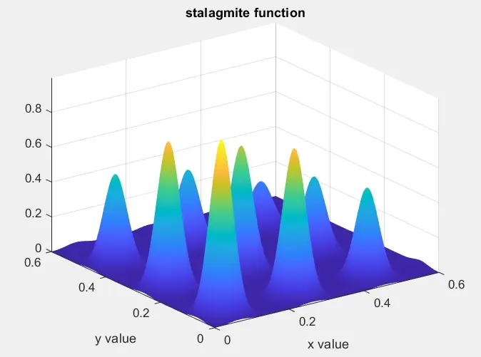
The above image shows the stalagmite form of output obtained using the “ga” function and stalagmite function.

Statistical study 1: unbounded:

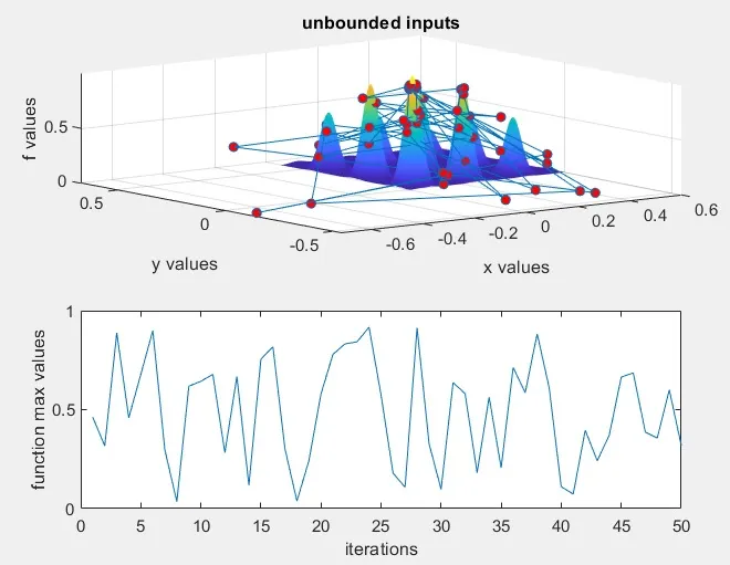
The above image is obtained as output for unbounded condition and it can be observed that points are not clear and variations in optimizing the function.

Statistical study 2: Bounded

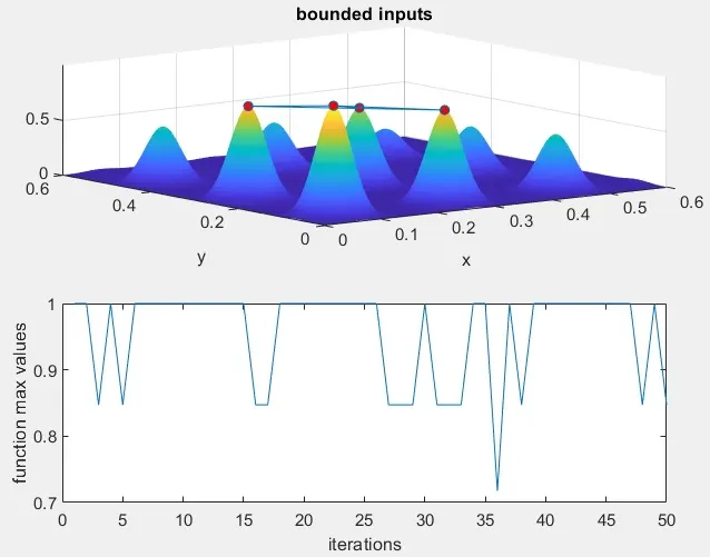
The above image shows the output for bounded condition, in this study a well-defined boundary is given in the “ga” function. From the output image, it can be observed that providing boundary, limits the variation in the optimum value.

Statistical study 3 with an increase in population:

In this study, the population study is increased using “optimoption” command, by increasing the population size, which leads to finding better fitness of the function.

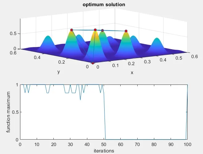
The above image shows the output of the study with increased population size.

Conclusion:

The Matlab code to optimize the stalagmite function and to find the global; maxima of the function is written and executed and corresponding results are achieved. The output shows better results when boundaries are defined.