Week 3 - Solving second order ODEs

Solving second order ODEs

Objective:

To write a program in order to solve ODE to acquire the position of the ball when functioned as a pendulum and to animate the position of the pendulum from obtained position information.

Given ODE

`d^2θ/dt^2 + (b/m)*dθ/dt + g/Lsin θ = 0`

where,

b = damping

m = mass, kg

g = gravity, m/s

L = length, m

Given parameters

Length = 1m

Mass = 1kg

Damping coefficient = 0.05

Gravity = 9.81m/s

Time period = 20s

Angular displacement = 0, angular velocity = 3rad/s, at t = 0

Matlab code for solving ODE

The MatLab file of solving ode challenge has been uploaded to the google drive and the access link to the file is

https://drive.google.com/file/d/1yw6NO0i3btwtvab3wR1N4-ntCaddb3o3/view?usp=sharing

clear all
close all
clc

%inputs
b = 0.05;
g = 9.81;
l = 1;
m = 1;

%initial conditions
theta_0 = [0;3];

%time points
t_span = linspace(0,20,300);

%solve ODE
[t,results] = ode45(@(t,theta)ode_func(t,theta,b,g,l,m),t_span,theta_0);

plot(t,results(:,1))
hold on
plot(t,results(:,2))
ylabel('plot')
xlabel('time')

fig = 1;
for i = 1:length(t)
    figure(1)
    %initial position
    x0 = 0;
    y0 = 0;
    %position of pendulum
    x1 = -l*sin(results(i,1));
    y1 = -l*cos(results(i,1));
    %plotting
    figure(2)
    %line for fixed support
    plot([-1 1],[0,0],'linewidth',3,'color','m');
    hold on
    %vertical line
    plot([x0 x1],[y0 y1],'linewidth',3,'color','b');
    %pendulum ball
    plot(x1,y1,'o','markersize',30,'markerfacecolor','r');
    axis([-2 2 -2 2]);
    pause(0.002);
    hold off
    M(fig) = getframe(gcf);
    fig = fig+1;
end
%for creating video and to store it in .avi format
movie(M)
videofile = VideoWriter('pendulum_video.avi','uncompressed AVI');
open(videofile)
writeVideo(videofile,M)
close(videofile)

Code description:

Input parameters such as length, mass, damping coefficient, gravity are given as input, initial condition values of angular displacement and angular velocity values such as 0 and 3rad/sec are given respectively.

The time period for the process is 20secs and it is given with the use of linspace command.

To solve second order differential equation an inbuilt ode function is called which is “ode45”, here we request another user established function which is saved as “ode_func” which accepts t, theta, b, g, l, m as input, which is programmed with the given ode equation of pendulum.

MatLab code of the declared function, ode_func

The MatLab file of the function code is uploaded to google drive and the access link to the file is

https://drive.google.com/file/d/1QadqoNkUU3h8rLWBaFXd3iJxtqhRjfkU/view?usp=sharing

%function code for solving ODE

function [dtheta_dt] = ode_func(t,theta,b,g,l,m)

theta1 = theta(1);
theta2 = theta(2);
dtheta1_dt = theta2;
dtheta2_dt = -(b/m)*theta2-(g/l)*sin(theta1);
dtheta_dt = [dtheta1_dt; dtheta2_dt];
end

Then plot command is used in order to plot the results obtained to obtain as output.

To create an animation video of the motion of the ball which functions as a pendulum, for the command is used. Here baseline, vertical line, ball position is defined.

Then the frames created are collected and created to a video file using video file command and saved as “pendulum video” in .avi format.

The animation video is uploaded to google drive and the access link to the file is

https://drive.google.com/file/d/1-6BvtepuTgtQQSXEyBOK6CXL5UDbZggK/view?usp=sharing

Results:

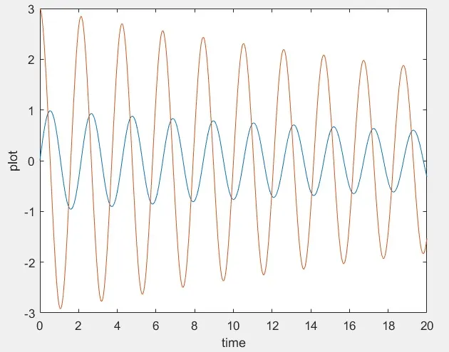
The above diagram represents the plot against time for the pendulum motion of the ball for a time period of 20secs.

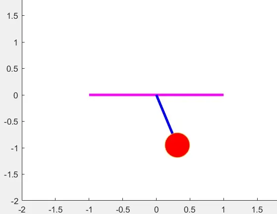
The above image shows a frame of animation of pendulum obtained by solving ode using MatLab.

Conclusion:

The ode equation for the pendulum is solved using MatLab code and animation of the ball motion is saved as a video file.