Week 4 - Genetic Algorithm
OPTIMISING THE STALAGMITE FUNCTION USING GENETIC ALGORITHM
Aim:
To optimise stalagmite function and find the global maxima of the given function using genetic algorithm approach in MATLAB.
Inputs:
Stalagmite function:`f = (f_(1x)*f_(1y)*f_(2x)*f_(2y))`
where,
`f_(1x)=[sin(5.1*pi*x+0.5)]^6`
`f_(1y) =[sin(5.1*pi*y+0.5)]^6`
`f_(2x)= e^((-4*log(2)*((x-0.667)^2//(0.64)))`
`f_(2y)= e^((-4*log(2)*((y-0.667)^2//(0.64)))`
Theory:
Stalagmite function:
This is one of the mathematical models that results in generation of maxima and minima. Global maxima are the highest value in the function and global minima is vice versa. This is a single value whereas the local minima and local maxima are multiple no. of values
Optimisation:
It is the process of finding the maxima and minima of a particular function.
Genetic algorithm:
This algorithm extracts the optimisation strategies and transform them for applications in the mathematical optimisation theories to find the global optimum at a defined space. Initially this creates a population with each sitting on the best place are selected and will reproduce thus creating a new population. The acceptable sections of two values recombine to give better values. Actually, many of these acceptable sections recombine forming new values are not successful but few will indeed fill the part.
Now as the recombination and forming the population with no new area exploration leads to premature convergence of the algorithm by missing the global optimum and only forming the local optimum. Hence the mutation process takes place where one can explore new areas of the algorithm and new population being formed up a little bit to get the new information into this set of section. This algorithm follows the biological gene process known as the Darwinian Evolution Algorithm. The following are the three-step process that takes place in this algorithm.
- Selection
- Mating/Crossover
- Mutation
In this algorithm, it generates many solutions forming a population. They are scored by objective or fitness function. they are combined so best is reproduced with best triad of previous solutions… this goes till it is satisfied. The genetic algorithm performance increases with the method chosen to encode the solution, probability of cross over and mutation, number of iterations and size of population.
Coding:
1: code for stalagmite function
%defining the function
function [f] = stalagmite(input_vector)
%variables in the function
x=input_vector(1)
y=input_vector(2)

f1_x=[sin(5.1*pi*x+0.5)]^6
f1_y=[sin(5.1*pi*y+0.5)]^6
f2_x=exp(-4*log(2)*((x-0.667)^2/(0.64)));
f2_y=exp(-4*log(2)*((y-0.667)^2/(0.64)));
%as GA generates only minimas by default, negative function
%has been considered for computing the maxima.
f= -(f1_x*f1_y*f2_x*f2_y);

end
2:code for optimisation
clear all
close all
clc
%defining the inputs variables
x= linspace(0,0.6,200);
y= linspace(0,0.6,200);
n=50
[xx yy] = meshgrid(x, y);

%generating the for loop to assign the values to the vectors

for i= 1:length(xx);
    for j=1:length(yy);
    input_vector(1)=xx(i,j);
    input_vector(2)=yy(i,j);
    f(i,j)=stalagmite(input_vector);

    end
end
%plotting the Stalagmite function
 figure(1)
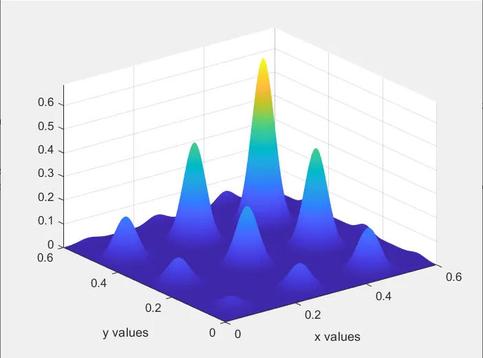
 surfc(xx,yy,-f)                    %surfc() generates the surface plot
 xlabel('x values')
 ylabel('y values')
 shading interp                     %this removes the lines on the surface plots

 [inputs, fval] = ga(@stalagmite,2) %introducing the GENETIC ALGORITHM

 %case 1
 %to calculate the Genetic Algorithm for limited iterations without any
 %specific boundraies


 tic                                %this starts the time interval.

 for m = 1:n
     [inputs,fopt(m)]=ga(@stalagmite,2)
     xopt(m)=inputs(1);
     yopt(m)=inputs(2);
 end


 studytime_1 =toc                   %stopping the time interval with studytime_1 name

 figure(2)
 subplot(2,1,1)                     %subplot() creats the second plot in the same window
 hold on
 surfc(x,y,-f)
 xlabel('x-values');
 ylabel('y-values');
 shading interp

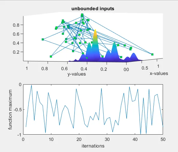
 plot3(xopt,yopt,-fopt,'marker','square','markersize',5,'markerfacecolor','g');
                                    %plot3() is used to plot the optimum value of the function generated with Genetic Algorithm
 title('unbounded inputs');
 subplot(2,1,2)
 plot(fopt)
 xlabel('iternations')
 ylabel('function maximum')


 %study_2
 %we include the boundries to the inputs in this case
 tic                                 %starting the time interval
 num_case = 50;                      % the no.of iterations to be carried out are defined


%generating the for loop for assigning the values
 for m = 1:num_case
     [inputs,fopt(m)]=ga(@stalagmite,2,[],[],[],[],[0:0],[0.6,0.6]);
%this is a syntax for GA for defining the boundaries.
     xopt(m)=inputs(1);
     yopt(m)=inputs(2);
 end


 study_time_2=toc;
 figure(3)
 subplot(2,1,1)
 hold on
 surfc(x,y,-f)
 xlabel('x-values');
 ylabel('y-values');
 shading interp
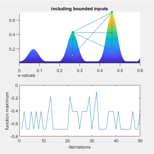
 plot3(xopt,yopt,-fopt,'marker','square','markersize',5,'markerfacecolor','g');
 title('including bounded inputs');
 subplot(2,1,2);
 plot(fopt);
 xlabel('iternations');
 ylabel('function maximum');


 %study-3 %we are introducing the population here for much optimization.

 options=optimoptions('ga'); %optimising the GA
options=optimoptions(options,'populationsize',300 );
tic                            %start of the interval


%generating the for loop for assigning the values
for l = 1:num_case
     [inputs,fopt(m)]=ga(@stalagmite,2,[],[],[],[],[0,0],[0.6:0.6],[],[],options);
%this is another syntax for GA for defining the boundaries with the population

     xopt(l)=inputs(1);
     yopt(l)=inputs(2);
 end


 study_time_3=toc               %stopping the interval
 figure(4)
 subplot(2,1,1)                 %subplot() creats the second plot in the same window
 hold on
 surfc(x,y,-f)
 xlabel('x-values');
 ylabel('y-values');
 shading interp
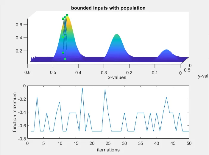
 plot3(xopt,yopt,-fopt,'marker','square','markersize',5,'markerfacecolor','g');
 title('bounded inputs with population');
 subplot(2,1,2);
 plot(fopt);
 xlabel('iternations');
 ylabel('function maximum');
Procedure:
- To find the global maxima of the stalagmite function, the function is coded in the MATLAB program. As the GA only provides the minima by default, the negative symbol is applied to the function.
- To study the Genetic Algorithm intensively, three study cases are performed.
- The linspace() command is used to provide the range for the input variables.
- The meshgrid command is used to convert the 2D arrays into 3D surface plots.
- Then the programmed stalagmite function is called out to calculate and output is directed to variable ‘f’.
- The surf command is used to draw the 3D with a solid edge colouring with shading interp command it maintains the shading of the formed surface by hiding the grind lines on the surface.
- In the first study no bound values and constraints are not assigned, where we get different values for each iteration it calculates.
- Tic and toc command used to calculate the execution time.
- The plot3() command is used to draw the 3D plot graph.
- In the study case 2, we assign certain bound conditions to the algorithm hence a different syntax has been used for the Genetic Algorithm.
Ga(@stalagmite,2,[],[],[],[],[0,0],[0.6,0.6]), where the empty braces represent to read the linear equality and inequality constraints and upper, lower bounds are provided.
- In the study case 3, we are providing the population value using the otimoptions command. The syntax for ga changes in this study as
ga(@stalagmite,2,[],[],[],[],[0,0],[0.6,0.6],[],[],options).
- Improved results are obtained by increasing number of iterations.
RESULT POLTS:
1: The stalagmite function
2: Using the Genetic Algorithm with unbounded values
3: with the bounded values
4: optimising with including the population to the algorithm
ERRORS:
1: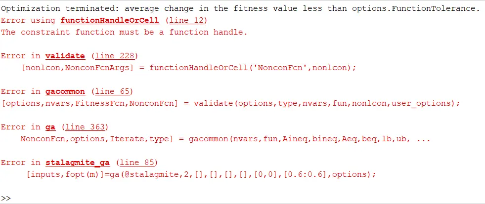
Rectification: the syntax for the ga function using for the population was incorrect, the syntax has been corrected and error has been rectificated.