Week 3 - Solving second order ODEs

Aim : To solve a second Order Differential Equation using MATLAB and to simulate the motion of pendulum using MATLAB.

Governing Equation:

`(d^2theta)/dt^2 + b/m*(d theta)/dt + g/lsintheta = 0`

Where:

b= damping coefficient

m= mass of the ball,

g= acceleration due to gravity,

l= length of string.

Inputs:

l = 1 meter

m= 1 kg

b= 0.05

g= 9.81`ms^2`

angular displacement = 0

angular velocity = 3 at time = 0

Theory:

Simple harmonic motion:

In general physics simple harmonic motion is said to a repetitive movement back and forth through as equilibrium or central position so that the max displacement on one side is equal to the other side. The time period of each complete motion is said to be same. The force responsible for this motion is always direct itself to the equilibrium position which is directly proportional to the distance from it.

The f is directly proportional to displacement in -ve direction.

Ex:

1. vibration of mass attached to vertical spring.
2. a simple pendulum.

For a simple pendulum, the dynamic behaviour of bob is crucial to understand. In engineering applications, the ODE is used to describe the behaviour of the system wrt time in term s of second order ODE. The movement of simple pendulum depends on newton’s second law of motion.

The equation of motion for a simple pendulum is,

`(d^2theta)/dt^2 + b/m*(d theta)/dt + g/lsintheta = 0`

We can breakdown this kind of 2^nd ODE into 1^st,

`(d theta_2)/dt = -b/mtheta_2 - g/lsintheta_1`

These equations can be written in form of matrix as,

`d/dt[ [theta_1] ,[theta_2]] =[[ theta_2] ,[-b/mtheta_2-g/lsintheta_1]]`

Code:

for defining the ode fuction

%defining the function of ODE

function [dtheta_dt] = ode_function(t,theta,b,m,g,l)

theta1=theta(1);
theta2 = theta(2);
dtheta1_dt = theta2;
dtheta2_dt = -(b/m)*theta2- (g/l)*sin(theta1);
dtheta_dt =[dtheta1_dt;dtheta2_dt];
end

for solving the ode function and simulation the pendulum motion

% MATLAB program for solving 2nd ODE
clear all;
close all;
clc;

%inputs
b =0.05
g = 9.81
l =1
m = 0.1

%initial conditions
theta_0 = [0;3];

%time interval to be calculated

t_span =linspace(0,20,550);

% calling ODE function
[t,results] = ode45(@(t,theta) ode_function(t,theta,b,m,g,l),t_span,theta_0);

% plotting the graph for angular displacement and angular velocity against
% time

figure(1)
plot(t,results(:,1));
hold on
plot(t,results(:,2));
hold off
axis([0 20 -3 4 ])
title("Graph for Angular Displacement and Angular Velocity");
xlabel("TIME");
ylabel("DISP&VEL");


% for animation the pendulum motion
%defining a counter initation for animation
ct = 1;
for i = 1:length(results(:,1))
    x0 = 0;
    y0 = 0;
    x1 = l*sin(results(i,1));
    y1 = -l*cos(results(i,1));
    
    
    plot([ -1 1],[0 0],'linewidth',3);
    line([ x0 x1],[y0 y1],'linewidth',3);
    hold on
    plot(x1, y1, "marker","o","markersize",20,"markerfacecolor",'g')
    axis([-2 2 -2 0.5])
    grid on 
    title("MOTION OF A PENDULUM")
    pause(0.01);
    M(ct) = getframe(gcf);
    ct = ct+1;
    hold off
end

movie(M)
videofile = VideoWriter("PENDULUM_MOVIE" , "uncompressed AVI");
open(videofile)
writeVideo(videofile,M)
close(videofile);
    

Procedure:

1. The ordinary differential equation of 2^nd order is converted into 1^st order and then into matrix form.
2. A MATLAB function is created namely ode_function which is a function of dtheta_dt
3. This function solves the ODE.
4. In a new program, all the inputs are mentioned b, g in m/s, l in meters, m in kg, and initial conditions at time interval zero where angular displacement and velocity as 0 and 3.
5. The duration of time is considered as 20 sec, using linspace it is divided into 550 equal parts for an accurate plot.
6. Later the function ‘ode_function’ is called out for solving the equation with ode45(@,,) function which is one of the inbuilt functions in Matlab.
7. A graph of time vs angular displacement ana angular velocity is plotted using plot() command, providing a title, xlabel and ylabel and an axis for it.
8. For visual simulation of the pendulum a counter initiative(ct) is defined and the length of the variable is defined.
9. As the pendulum is said to be at mean position during the starting of simulation the x0 and yo are given as (0,0).
10. As the pendulum moves and the forces act on it, the position the pendulum is given in terms of theta.
11. Defining the rigid support using line command and length of the pendulum with (marker, markersize) commands.
12. The title, axis and the pause intervals are also defined for better visualization.
13. The animation created and saved my the movie(M),VideoWriter commands and providing the format of the video.

errors:

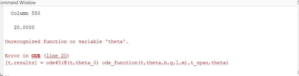
rectification: the function theta_0 was not entered properly and re-entered and corrected the mistake.

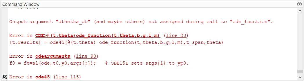
rectification: the spelling of theta was entered incorectly ans recorrected by enetring by right spelling.

Output Plots:

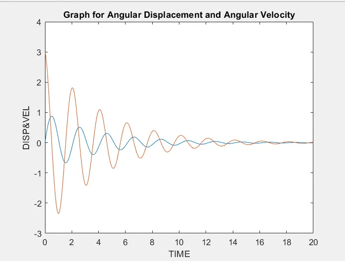
animation file: https://drive.google.com/file/d/1dcqkjnggQ9aojxgv0ewU6Zv_QI6tLKHF/view?usp=sharing

Conclusion:

the simulation of the simple pendulum using ODE is calulated and animated, an related graphs are plotted.