Project 2 - Rankine cycle Simulator

RANKINE CYCLE SIMULATOR

Aim:

To calculate the state points of a Rankine cycle by plotting the T-S, H-S plots from given input variables.

Inputs:

1. Turbine inlet temperature = 400 Celsius
2. Turbine inlet pressure = 30 bars
3. Turbine outlet pressure = 0.05 bars

Assumptions:

The cycle has been considered as an ideal rankine cycle

Theory:

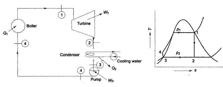
Rankine cycle consists of a turbine, condenser, pump and a boiler, it consists of following processes

1-2: isentropic expansion in the turbine

2-3: constant pressure heat rejection

3-4: isentropic compression

4-1: constant pressure heat addition

Procedure:

The process: (1-2) takes place in turbine where the steam from the boiler enters the turbine having high temperature and pressure, the steam expands in the turbine producing the work and then sent to the condenser.

The process: (2-3) takes place in the condenser where the steam from the turbine is condensed to the liquid water medium and sent to the pump.

The process: (3-4) takes place in the pump where it pressurizes the liquid before gong the boiler.

The process: (4-1) where the pressurized liquid enters the boiler and is heated to super-heated steam, here work is added to the system.

Code:

%RANKINE CYCLE SIMULATOR
%INPUTS temp =400, pressure_in = 0.05, pressure_out = 3;
clear all
close all
clc

%inputs
fprintf('%75s', 'Rankine Cycle Simulator');
fprintf('\n\n\n')
fprintf('1-2 is isentropic expansion which takes place in turbine \n');
fprintf('2-3 is constant pressure heat rejection in condenser \n');
fprintf('3-4 is isentropic compressoin takes place in pump /n');
fprintf('4-1 is constant presure heat addition in the boiler \n');

% given inputs
p1 = input('enter the value of pressure(bar) at state-1(inlet of turbine):');
t1 = input('enter the value of temperature(degrees) at state-1(inlet of turbine):');
p2 = input('enter the value of pressure(bar) at state-2(inlet of condensor):');



%% inputs from XSteam

%% at turbine
s1 = XSteam('s_pt',p1,t1);
h1 = XSteam('h_pt',p1,t1);

%% at condensor
% during (1-2) as it is isentropic expansion the entropy doesnt change
s2   = s1;
sf2  = XSteam('sL_p',p2);
sg2 = XSteam('sV_p',p2);
hf2  = XSteam('hL_p',p2);
hg2 = XSteam('hV_p',p2);

% dryness fraction(x)

if(s2<=sg2)
    x2 = ((s2-sf2) /(sg2-sf2));
else
    x2 =1;
end

h2=hf2+(x2*(hg2-hf2));

% at exit of the condensor
p3 = p2;
t3 = XSteam('Tsat_p',p3);
s3 = XSteam('sL_p',p3);
h3 = XSteam('hL_p',p3);
v3 = XSteam('vL_p',p3);
t2 = t3;

%% At the inlet of boiler
%  As it is an isentropic compression and constant heat addition takes
%  place in the boiler p4=p1 & s4 = s3

p4  = p1;
s4  = s3;
h4  = XSteam('h_ps',p4,s4);
cp4 = XSteam('Cp_ps',p4,s4);
cv4 = XSteam('Cv_ps',p4,s4);

gamma4 = (cp4/cv4)
% we know that 
%p_a^(1-gamma)*t_a*gamma = p_b^((1-gamma)/gamma)

t4 = (t3*((p3/p4)^((1-gamma4)/gamma4)));

%%  work and efficeincy calculations

%  1:work done by the turbine
w_t = h1 - h2;

%  2:work done by the pump

w_p = h4 - h3; 
%  3:total work done by the system 
w_net = w_t - w_p;



%where
%q_in is heat addition in the boiler

q_in = h1 - h4;


% q_out is heat rejection in the condensor

q_out = h2 - h3;



% thermal efficiecy 

eta = (w_net/q_in)*100;





%% plotting the H-S and T-S diagrams

%% plotting T-S diagram
 figure(1)
% plotting liquid and vapour curves
t          = linspace(1, t1, 1000);
for i      = 1:length(t)
    s_l(i) = XSteam('sL_T',t(i));
end

for i = 1:length(t)
    sat_vap(i) = XSteam('sV_T',t(i));
end
hold on 
plot(s_l,t,'linewidth',3,'linestyle','-.','color','m')

plot(sat_vap,t,'linewidth',3,'linestyle','-.','color','m')
grid off

% for the process (1-2)
plot([s1,s2],[t1,t2],'linewidth',3,'color','k')
hold on
% for the process(2-3)
plot([s2,s3],[t2,t3],'linewidth',3,'color','k')
hold on
% for the process(3-4)
plot([s3,s4],[t3,t4],'linewidth',3,'color','k')
hold on 

% for the process(4-1)
tp = XSteam('TSat_p',p4);
sp = XSteam('sL_T',tp);
plot([s4,sp],[t4,tp],'linewidth',3,'color','k')
hold on

% for
tq = tp;
sq = XSteam('sV_T',tq);
plot([sp,sq],[tp,tq],'linewidth',3,'color','k')
hold on 


plot([sq,s1],[tq,t1],'linewidth',3,'color','k')
hold on 

title('T-S DIAGRAM OF IDEAL RENKINE CYCLE')
xlabel('ENTROPY(KJ/KgK)')
ylabel('TEMPERATURE(K)')

% mentioning the process states with numericals
text(s1,t1,'1');
text(s2,t2,'2');
text(s3,t3,'3');
text(s4,t4,'4');

%% plotting the diagram of H-S

figure(2)

% plotting liquid and vapour curves
t          = linspace(1, t1, 1000);
for j      = 1:length(t)
    h_l(j) = XSteam('hL_T',t(j));
end

for j = 1:length(t)
    h_vap(j) = XSteam('hV_T',t(j));
end
hold on 
plot(s_l,h_l,'linewidth',3,'linestyle','-.','color','m')
hold on
plot(sat_vap,h_vap,'linewidth',3,'linestyle','-.','color','m')
grid off


%at prosess(1-2)
plot([s1,s2],[h1,h2],'linewidth',3,'color','k')
hold on

%at prosess(2-3)
plot([s2,s3],[h2,h3],'linewidth',3,'color','k')
hold on

%at prosess(3-4)
plot([s3,s4],[h3,h4],'linewidth',3,'color','k')
hold on


%at prosess(4-1)
plot([s4,s1],[h4,h1],'linewidth',3,'color','k')

title('H-S DIAGRAM OF IDEAL RENKINE CYCLE')
xlabel('ENTROPY(KJ/KgK)')
ylabel('ENTHALPY(KJ/KgK)')

% mentioning the process states with numericals
text(s1,h1,'1');
text(s2,h2,'2');
text(s3,h3,'3');
text(s4,h4,'4');

%% OUTPUT TO BE DISPALYED

fprintf('%50s \n  \n \n','RESULT');
fprintf('%10s %60s \n','At point-1','At point-2');
fprintf('%s %.2f %s %44s %.2f%s \n','P1:',p1,'bar','P2:',p2,'bar');
fprintf('%s %.2f %s %35s %.2f%s \n','T1:',t1,'Deg celcious','T2:',t2,'deg celius');
fprintf('%s %.2f %s %40s %.2f%s \n','H1:',h1,'KJ/Kg','H2:',h2,'KJ/kg');
fprintf('%s %.2f %s %42s %.2f%s \n','S1:',s1,'KJ/KgK','S2:',s2,'KJ/KgK');

fprintf('%58s %.2f \n \n','X2:',x2);

fprintf('%10s %54s \n','At point-3','At point-4');
fprintf('%s %.2f %s %45s %.2f%s \n','P3:',p1,'bar','P4:',p4,'bar');
fprintf('%s %.2f %s %35s %.2f%s \n','T1:',t1,'Deg celcious','T4:',t4,'deg celius');
fprintf('%s %.2f %s %41s %.2f%s \n','H3:',h1,'KJ/Kg','H4:',h4,'KJ/kg');
fprintf('%s %.2f %s %42s %.2f%s \n','S3:',s3,'KJ/KgK','S4:',s4,'KJ/KgK');


%other parameters

fprintf('%40s %.2f %s \n','work done by  the turbine(w_t):','wt','KJ/Kg');

fprintf('%40s %.2f %s \n','work done by  the pump(w_p):','wp','KJ/Kg');

fprintf('%40s %.2f %s \n','net  work (wnet):','wt','KJ/Kg');

fprintf('%40s %.2f %s \n','thermodynamic efficeincy (Ntherm):',eta,'percent');

fprintf('%40s %.2f %s \n','heat input in boiler:','q_in','KJ/Kg');

fprintf('%40s %.2f %s \n','heat rejection by condenser:','q_out','KJ/Kg');

fprintf('%40s %.2f %s \n','S.S.C:','p3','KJ/KWh');

RESULT:

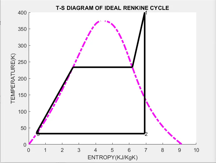
1: T-S DIAGRAM

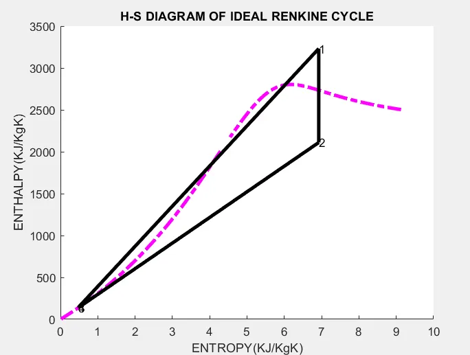
2: H-S DIAGRAM

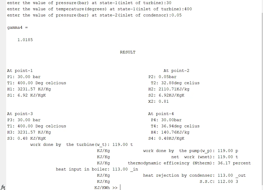
3: DISPLAYING THE RESULTS AND CALCULATED OUTPUTS:

Errors and corrections:

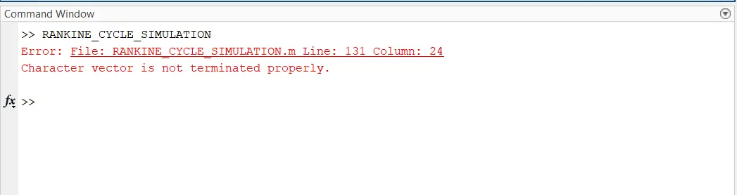
1 a vector has been present in the code line which has been mistakenly is typed.

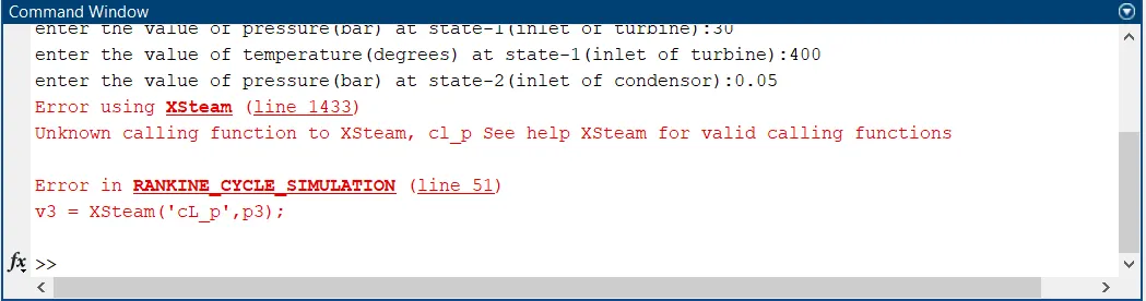
2: instead of entropy(s) typing error of (c) in place of (s) led to the error.

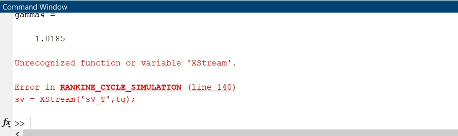
3: typing error while callin the function file XSteam :

Report:

1. For the ease of code, the cycle has been considered as an ideal rankine cycle where the heat transfer and the energy balance in the tubine and the pump can be neglected.
2. The execution and calculations of state points in the cycle have been simulated using the XSteam library provided.
3. firstly the enthalpy and entropy at state-1 (h1,s1) are been calculated with the given inputs and XSteam library.
4. then the t2, h2 and s2 are calculated from state-1 using XSteam.m.
5. the thermal efficiency , work done in the turbine, work done by the pump, heat input and oulet are calculated basing the states(1-2-3-4)
6. later with all the state points the T-S and H-S diagrams are plotted showing the processes 1-2, 2-3, 3-4 and 4-1.