Week 4 - Genetic Algorithm
Aim:
Write a code in Matlab store optimise the stalagmite function and find the global maximum of the function
Objective:
1. To write a code in metal apps to optimise the stalagmite function and find the global maximum of the function
2. The plot graphs for all three studios and for maximum number of iteration
Theory:
* Genetic algorithm is search-Based Optimisation technique based on the principle of genetic and natural selection it is frequently used to find optimal or a near optimal solution to difficult problems which otherwise would take a lifetime to Solve it is frequently. Used to solve optimisation problems in research and in machine learning.
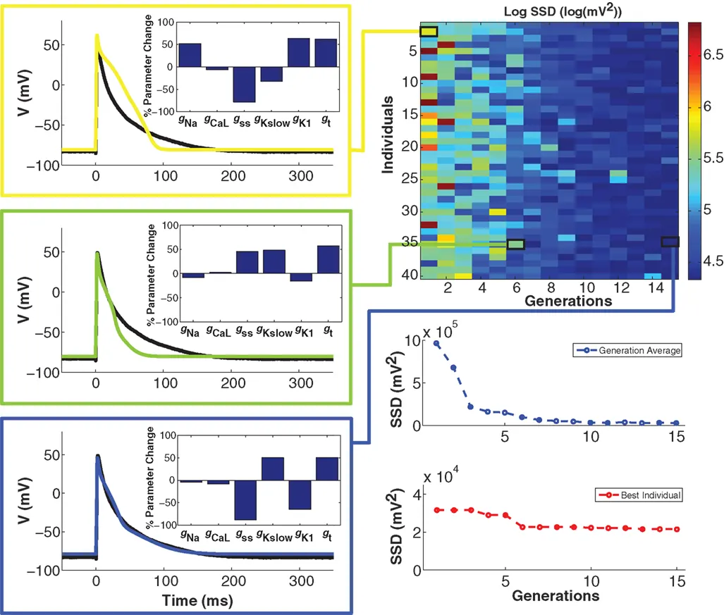
* A genetic algorithm is a search heuristic that is inspired by Charles Darwin’s theory of natural evolution. This algorithm reflects the process of natural selection where the fittest individuals are selected for reproduction in order to produce offspring of the next generation.
Notion of Natural Selection:
The process of natural selection starts with the selection of fittest individuals from a population. They produce offspring which inherit the characteristics of the parents and will be added to the next generation. If parents have better fitness, their offspring will be better than parents and have a better chance at surviving. This process keeps on iterating and at the end, a generation with the fittest individuals will be found.
This notion can be applied for a search problem. We consider a set of solutions for a problem and select the set of best ones out of them.
Five phases are considered in a genetic algorithm.
1.Initial population
2.Fitness function
3.Selection
4.Crossover
5.Mutation
Initial Population:
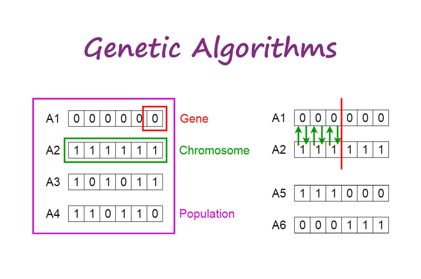
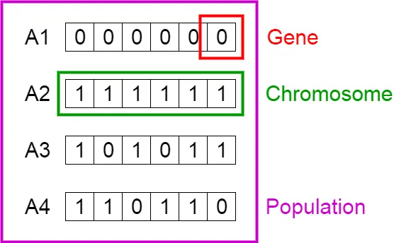
The process begins with a set of individuals which is called a Population. Each individual is a solution to the problem you want to solve.
An individual is characterized by a set of parameters (variables) known as Genes. Genes are joined into a string to form a Chromosome (solution).
In a genetic algorithm, the set of genes of an individual is represented using a string, in terms of an alphabet. Usually, binary values are used (string of 1s and 0s). We say that we encode the genes in a chromosome.
Fitness Function:
The fitness function determines how fit an individual is (the ability of an individual to compete with other individuals). It gives a fitness score to each individual. The probability that an individual will be selected for reproduction is based on its fitness score.
Selection:
The idea of selection phase is to select the fittest individuals and let them pass their genes to the next generation.
Two pairs of individuals (parents) are selected based on their fitness scores. Individuals with high fitness have more chance to be selected for reproduction.
Crossover: Crossover is the most significant phase in a genetic algorithm. For each pair of parents to be mated, a crossover point is chosen at random from within the genes.
For example, consider the crossover point to be 3 as shown below.
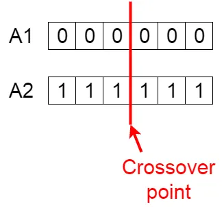
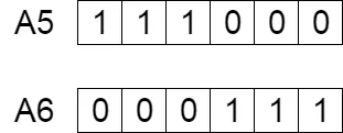
Offspring are created by exchanging the genes of parents among themselves until the crossover point is reached.
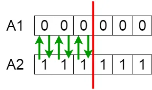
The new offspring are added to the population.
Mutation:
In certain new offspring formed, some of their genes can be subjected to a mutation with a low random probability. This implies that some of the bits in the bit string can be flipped.
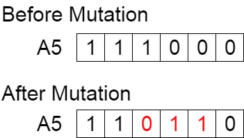
Mutation occurs to maintain diversity within the population and prevent premature convergence.
Termination:
The algorithm terminates if the population has converged (does not produce offspring which are significantly different from the previous generation). Then it is said that the genetic algorithm has provided a set of solutions to our problem.
Advantages of genetic algorithm:
1. there does not require any derivative information(Which may not be available for many real-world problems)
2. Genetic algorithm is faster and more efficient as compare to traditional methods.
3. Genetic algorithm has very good parallelcapabilities.
4. Genetic algorithm optimise both continuous and discrete function and also multi-Objective problems.
5. Genetic algorithm provides a list of good solution and not just a single solution.
6. Genetic algorithm always gets answer to the problem which gets better over the time.
7. Genetic algorithm is useful when the search space is very large and there are a large number of parametres involved.
Limitation of Genetic Algorithm:
1. Genetic algorithm or not suited for all problems especially problems which are simple and for which derivatives information is available.
2. The fitness value is calculated repeatedly which might be computationally expensive for some problems.
3. Bing stochastic dear or no guarantee on the optimality or the quality of the solution.
4. If not implemented properly the genetic algorithm may not coverage for the optimal solution.
What is Traditional Algorithm:
Traditional Algorithms refers to general algorithms we use to solve problems. It is a methodical procedure to solve a given problem. There can be several algorithms to solve a problem. Therefore, it is important to analyze each and find the required time, space etc. to select the best algorithm to solve the problem.
A traditional algorithm must be clear. It should have 0 or more number of well-defined inputs and 1 or more well-defined outputs. It should also be capable of finding solutions with available resources. Furthermore, it should complete the task after some finite number of steps.

Following are some common traditional algorithms.
Search – These algorithms help to search a particular item in a data structure. (Linear search, Binary search)
Sort – These algorithms help to sort a set of elements in a specific order. (Bubble sort, Selection sort, Insertion sort)
Divide and Conquer – It refers to dividing a large problem into small subproblems and solving the subproblems in order to find the solution to the original problem.
Difference Between Genetic Algorithm and Traditional Algorithm
Definition
Genetic algorithm is an algorithm for solving both constrained and unconstrained optimization problems that are based on Genetics and Natural Selection while traditional algorithm is an unambiguous specification that defines how to solve a problem. Thus, this is the main difference between genetic algorithm and traditional algorithm.
Usage
The specific use of each algorithm is an important difference between genetic algorithm and traditional algorithm. That is; the genetic algorithm helps to find the optimal solutions for difficult problems while traditional algorithm provides a step by step methodical procedure to solve a problem.
Complexity
Another difference between genetic algorithm and traditional algorithm is that a genetic algorithm is more advanced than a traditional algorithm.
Applications
Genetic Algorithm is used in fields such as research, Machine Learning and, Artificial Intelligence. Traditional algorithm is used in fields such as Programming, Mathematics, etc. Hence, this is also an important difference between genetic algorithm and traditional algorithm.
Conclusion
In addition to traditional algorithms, there is a special type of algorithm called genetic algorithms. The main difference between genetic algorithm and traditional algorithm is that genetic algorithm is a type of algorithm that is based on the principle of genetics and natural selection to solve optimization problems while traditional algorithm is a step by step procedure to follow, in order to solve a given problem. Searching, sorting algorithms etc. are traditional algorithms while genetic algorithms are more complex and used in areas such as artificial intelligence and research.
Difference Between classic algorith and genetic algorithm.
| Classical Algorithm | Genetic Algorithm |
|---|---|
| Generates a single point at each iteration. The sequence of points approaches an optimal solution. | Generates a population of points at each iteration. The best point in the population approaches an optimal solution. |
| Selects the next point in the sequence by a deterministic computation. | Selects the next population by computation which uses random number generators. |
Governing Equations:
`rightarrow` `f(x,y) = f1,x * f2,x * f1,y *f2,y`
`rightarrow` `f1,x = (sin(5.1pix + 0.5))^6`
`rightarrow` `f1,y = (sin(5.1pix+0.5))^6`
`rightarrow` `f2,x = exp(-4ln(2)((x - 0.0667)^2 /(0.64)))`
`rightarrow` `f2,y = exp(-4ln(2)((y - 0.0667)^2 /(0.64)))`
Syntax in 'ga' in Matlab's:
x = ga(fun,nvars)x = ga(fun,nvars,A,b)x = ga(fun,nvars,A,b,Aeq,beq)x = ga(fun,nvars,A,b,Aeq,beq,lb,ub)x = ga(fun,nvars,A,b,Aeq,beq,lb,ub,nonlcon)x = ga(fun,nvars,A,b,Aeq,beq,lb,ub,nonlcon,options)x = ga(fun,nvars,A,b,[],[],lb,ub,nonlcon,IntCon)x = ga(fun,nvars,A,b,[],[],lb,ub,nonlcon,IntCon,options)x = ga(problem)[x,fval] = ga(___)
Description:
x= ga(fun,nvars)x, to the objective function,fun.nvarsis the dimension (number of design variables) offunx= ga(fun,nvars,A,b)xtofun, subject to the linear inequalitiesA*x≤b.gaevaluates the matrix productA*xas ifxis transposed (A*x').x= ga(fun,nvars,A,b,Aeq,beq)xtofun, subject to the linear equalitiesAeq*x=beqandA*x≤b. (SetA=[]andb=[]if no linear inequalities exist.)gaevaluates the matrix productAeq*xas ifxis transposed (Aeq*x').x= ga(fun,nvars,A,b,Aeq,beq,lb,ub)x, so that a solution is found in the rangelb≤x≤ub. (SetAeq=[]andbeq=[]if no linear equalities exist.)x= ga(fun,nvars,A,b,Aeq,beq,lb,ub,nonlcon)nonlcon. The functionnonlconacceptsxand returns vectorsCandCeq, representing the nonlinear inequalities and equalities respectively.gaminimizes thefunsuch thatC(x)≤0andCeq(x) = 0. (Setlb=[]andub=[]if no bounds exist.)x= ga(fun,nvars,A,b,Aeq,beq,lb,ub,nonlcon,options)options. (Setnonlcon=[]if no nonlinear constraints exist.) Createoptionsusingoptimoptions.x= ga(fun,nvars,A,b,[],[],lb,ub,nonlcon,IntCon)x= ga(fun,nvars,A,b,[],[],lb,ub,nonlcon,IntCon,options)IntContake integer values.x= ga(problem)problem, whereproblemis a structure.[, for any previous input arguments, also returnsx,fval] = ga(___)fval, the value of the fitness function atx.[also returnsx,fval,exitflag,output] = ga(___)exitflag, an integer identifying the reason the algorithm terminated, andoutput, a structure that contains output from each generation and other information about the performance of the algorithm.[also returns a matrixx,fval,exitflag,output,population,scores] = ga(___)population, whose rows are the final population, and a vectorscores, the scores of the final population.
Matlab Code:
Code containing stalagmite function.
function[f] = stalagmite(input_vector)

x = input_vector(1);
y = input_vector(2);

f_1_x = (sin(5.1*pi*x + 0.5)).^6;
f_1_y = (sin(5.1*pi*y + 0.5)).^6;
f_2_x = exp(-4*log(2)*(((x-0.0667)^2)/0.64));
f_2_y = exp(-4*log(2)*(((y-0.0667)^2)/0.64));
[f] = -((f_1_x)*(f_2_x )*(f_1_y)*(f_2_y));
end
Main code containing first study:
% a program to calculate the maxima of the functionwith unbounded inputs

clear all
close all
clc
%inputs for search space

x = linspace(0,0.6,150);
y = linspace(0,0.6,150);
num_cases = 50;


% creating a 2_dimensional mesh
[xx,yy] = meshgrid(x,y);


% evaluating the stalagmite function

for i=1:length(xx)
    for j=1:length(yy)
        input_vector(1) = xx(i,j);
        input_vector(2) = yy(i,j);
        f(i,j) = stalagmite(input_vector);
    end
end
tic
% study1-statistical behaviour with unbounded input values

for a=1:num_cases
    [input,fopt_1(a)] = ga(@stalagmite,2);
    xopt(a) = input(1);
    yopt(a) = input(2);
end

study1_time=toc

% plotting our data

figure(1)
subplot(2,1,1)
hold on
surfc(x,y,-f)
shading interp
colorbar
plot3(xopt,yopt,-fopt_1,'marker','o','markerfacecolor','r','markersize',5)
title('unbound inputs')
subplot(2,1,2)
plot(-fopt_1)
xlabel('Iterations')
ylabel('Function maxima')
Main code containing second study:
% a program to calculate the maxima of the function with bounded inputs

clear all
close all
clc
%inputs for search space

x = linspace(0,0.6,150);
y = linspace(0,0.6,150);
num_cases = 50;


% creating a 2_dimensional mesh
[xx,yy] = meshgrid(x,y);


% evaluating the stalagmite function

for i=1:length(xx)
    for j=1:length(yy)
        input_vector(1) = xx(i,j);
        input_vector(2) = yy(i,j);
        f(i,j) = stalagmite(input_vector);
    end
end
tic
% study1-statistical behaviour with uper and lower bounded inputs values


for b=1:num_cases
    [input,fopt_2(b)] = ga(@stalagmite,2,[],[],[],[],[0;0],[1;1]);
    xopt(b) = input(1);
    yopt(b) = input(2);
end

study2_time=toc

% plotting our data

figure(2)
subplot(2,1,1)
hold on
surfc(x,y,-f)
shading interp
colorbar
plot3(xopt,yopt,-fopt_2,'marker','o','markerfacecolor','r','markersize',5)
title('bounded inputs')
subplot(2,1,2)
plot(-fopt_2)
xlabel('Iterations')
ylabel('Function maxima')
Main code containing third study:
% a program to calculate the maxima of the function with bounded inputs and
% increasing iterations

clear all
close all
clc
%inputs for search space

x = linspace(0,0.6,150);
y = linspace(0,0.6,150);
num_cases = 50;


% creating a 2_dimensional mesh
[xx,yy] = meshgrid(x,y);


% evaluating the stalagmite function

for i=1:length(xx)
    for j=1:length(yy)
        input_vector(1) = xx(i,j);
        input_vector(2) = yy(i,j);
        f(i,j) = stalagmite(input_vector);
    end
end
tic
% study1-statistical behaviour with upper and lower bounded input values
% and increasing genetic algorithm iterations
option_1 = optimoptions('ga');
option_1 = optimoptions(option_1,'populationsize',300);


for c=1:num_cases
    [input,fopt_3(c)] = ga(@stalagmite,2,[],[],[],[],[0;0],[1;1],[],[],option_1);
    xopt(c) = input(1);
    yopt(c) = input(2);
end

study3_time=toc

% plotting our data

figure(3)
subplot(2,1,1)
hold on
surfc(x,y,-f)
shading interp
colorbar
plot3(xopt,yopt,-fopt_3,'marker','o','markerfacecolor','r','markersize',5)
title('bounded inputs with increasing population')
subplot(2,1,2)
plot(-fopt_3)
xlabel('Iterations')
ylabel('Function maxima')
Code Explaination:
1.Clear all clear all the variables in theworkspace.
2. Close all close all the plots and figures.
3. CLC clear the common window.
4. Linspace(0,0.6,150) creates 150 values between zero and 0.6 which are equally spaced. The array 1-D.
5. The meshgrid command transformers the domain specified by vector X and Y into array X and Y(2D).
6. The num_cases=50 Number of cases is set as 50.
7. For loop is executed to obtain the function values a different coordinates.
8. The function is called stalagmite function.
9. In case of study 1 genetic algorithm is used inside the for loop.
10. Tic and tok function is used to calculate the study time. Tic Start a stopwatch timer and Toc Prints the elapsed time since tic was used.
11. The subplot command Is used to plot two plots in a single figure window. 1 subplot command is used to display the curve Stalagmite Function along with the optimisation point. The 2 subplot command Is used to display the plot of number of iteration versus function maximum.
12. The surfc Command is used to generate the 3-D surface.
13. The shading interp Command is used to remove the grid lines from the 3-D surface and create a smooth shading.
14. The plot3 function displays a three-dimensional plot with set of data points.
15. Title command is used to give title name to the figure.
16. The commands X label and ylabel are used to name the X axis and Y axis.
Outputs:
study1_time:
in this case the randomness of the plots created by the stalagmite function using genetic algorithm can be observed.
study1_time =

    2.5721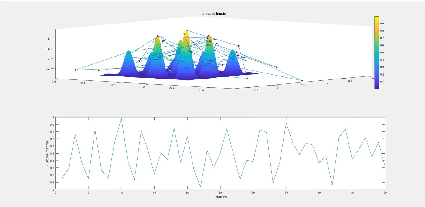
study2_time =

    3.3471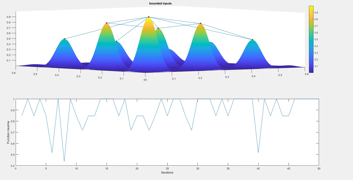
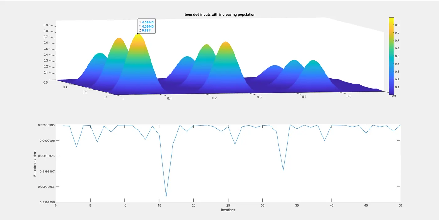
study3_time:
in this case the covergence of the data to one final value of the global maxima as opposed to a local maxima is obtained this value can be seen from the graph that has convered after varying the population size and however to value of 1.
study3_time =

   13.3886
REFERENCE: