Otto Cycle
AIM: Air standard Cycle.
Introduction:The Otto Cycle, describes how heat engines turn gasoline into motion. Like other thermodynamic cycles, this cycle turns chemical energy into thermal energy and then into motion. The Otto cycle describes how internal combustion engines (that use gasoline) work, like automobiles and lawn mowers.
Application:
The Otto Cycle provides the energy for most transportation and was essential for the modern world. Specifically, the vast majority of automobiles seen on the road today use the Otto Cycle to convert gasoline into motion. Any machine that uses gasoline will be divided into two categories of engines as seen below.
Types of engines that use the Otto Cycle
Figure 1. A two stroke engine
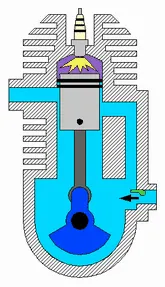
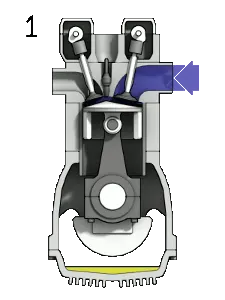
Figure 2. A four stroke engine
The engines' pages will provide details on their unique mechanisms, and an explanation on how they use the Otto Cycle, which is slightly modified.
The process of This Cycle is As Follow:
- Process 0–1 a mass of air is drawn into piston/cylinder arrangement at constant pressure.
- Process 1–2 is an adiabatic (isentropic) compression of the charge as the piston moves from bottom dead center (BDC) to top dead center (TDC).
- Process 2–3 is a constant-volume heat transfer to the working gas from an external source while the piston is at top dead center. This process is intended to represent the ignition of the fuel-air mixture and the subsequent rapid burning.
- Process 3–4 is an adiabatic (isentropic) expansion (power stroke).
- Process 4–1 completes the cycle by a constant-volume process in which heat is rejected from the air while the piston is at bottom dead center.
- Process 1–0 the mass of air is released to the atmosphere in a constant pressure process.
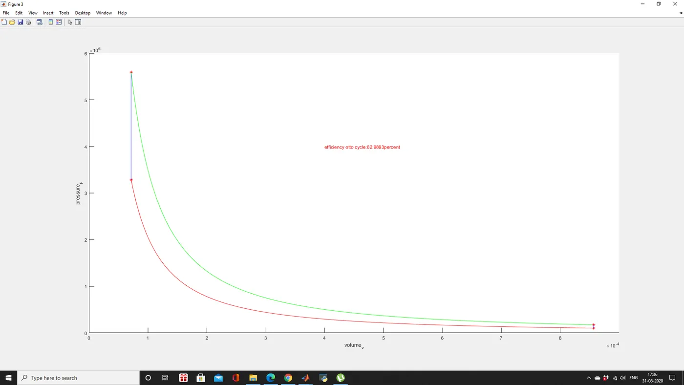
The pressure-volume diagram of an ideal Otto Cycle process. It consists of two isochoric, two adiabatic and two isobaric processes (for intake and exhaust)
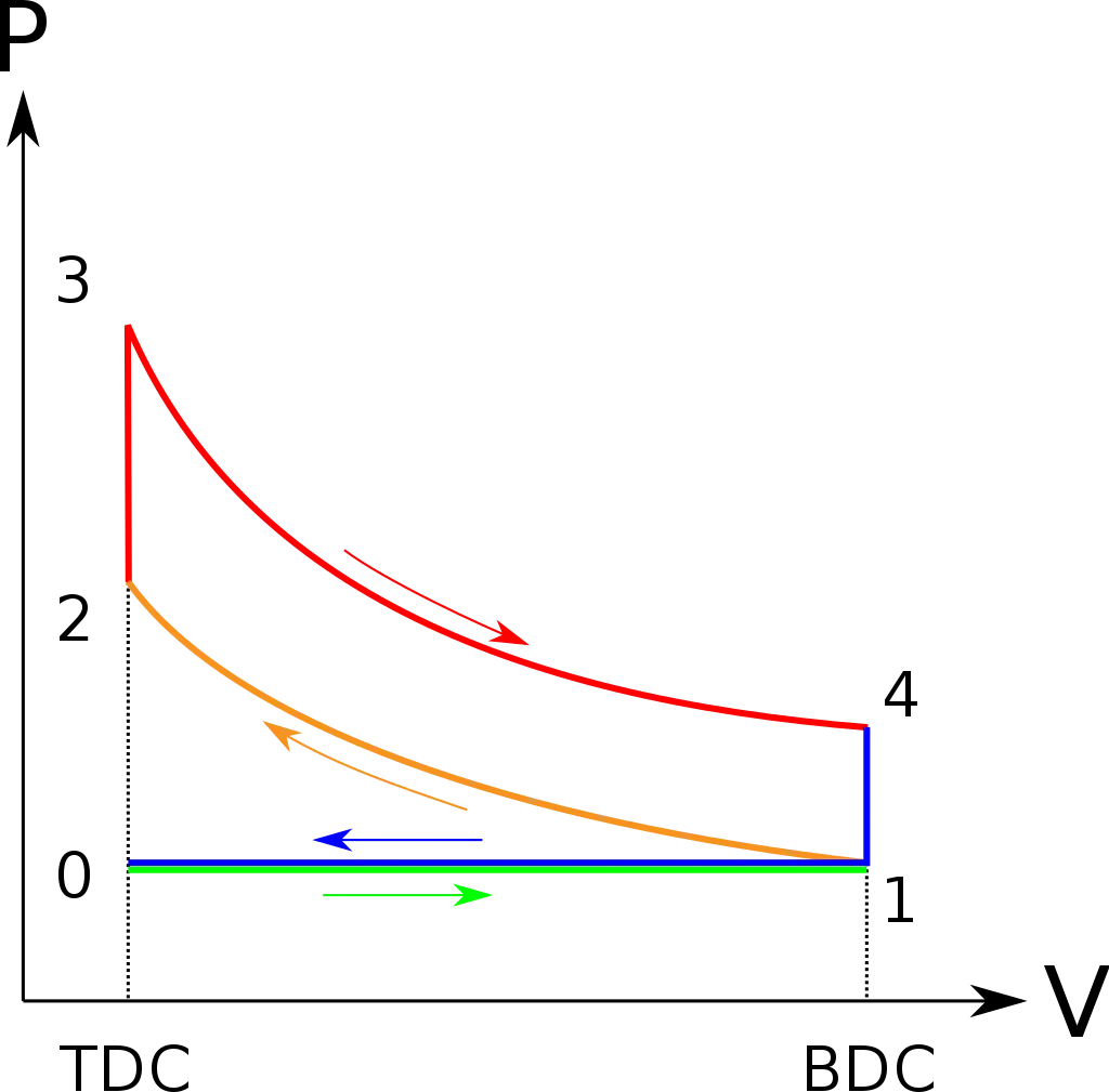
Process 0–1 intake stroke (Blue Shade)
A mass of air (working fluid) is drawn into the cylinder, from 0 to 1, at atmospheric pressure (constant pressure) through the open intake valve, while the exhaust valve is closed during this process. The intake valve closes at point 1.
Process 1–2 compression stroke
Piston moves from crank end (BDC, bottom dead centre and maximum volume) to cylinder head end (TDC, top dead centre and minimum volume) as the working gas with initial state 1 is compressed isentropically to state point 2, through compression ratio (V1/V2). Mechanically this is the isentropic compression of the air/fuel mixture in the cylinder, also known as the compression stroke. This isentropic process assumes that no mechanical energy is lost due to friction and no heat is transferred to or from the gas, hence the process is reversible. The compression process requires that mechanical work be added to the working gas. Generally the compression ratio is around 9–10:1 (V1:V2) for a typical engine.
Process 2–3 ignition phase
The piston is momentarily at rest at TDC. During this instant, which is known as the ignition phase, the air/fuel mixture remains in a small volume at the top of the compression stroke. Heat is added to the working fluid by the combustion of the injected fuel, with the volume essentially being held constant. The pressure rises and the ratio P3/P2 is called the "explosion ratio".
Process 3–4 expansion stroke
The increased high pressure exerts a force on the piston and pushes it towards the BDC. Expansion of working fluid takes place isentropically and work is done by the system on the piston. The volume ratio V4/V3 is called the "isentropic expansion ratio". (For the Otto cycle is the same as the compression ratio V1/V2. Mechanically this is the expansion of the hot gaseous mixture in the cylinder known as expansion (power) stroke.
Process 4–1 idealized heat rejection
The piston is momentarily at rest at BDC. The working gas pressure drops instantaneously from point 4 to point 1 during a constant volume process as heat is removed to an idealized external sink that is brought into contact with the cylinder head. In modern internal combustion engines, the heat-sink may be surrounding air (for low powered engines), or a circulating fluid, such as coolant. The gas has returned to state 1.
Process 1–0 exhaust stroke
The exhaust valve opens at point 1. As the piston moves from "BDC" (point 1) to "TDC" (point 0) with the exhaust valve opened, the gaseous mixture is vented to the atmosphere and the process starts anew.
clear all
close all
clc
%input
gamma=1.4;
t3=2300

% state variable
p1=101325
t1=500

% engine geometric
bore=0.1;
stroke=0.1;
con_rod=0.15; %connecting rod
cr=12;    %compression ratio cr = v1/v2


% calculating the swept volume and the clearrance volume

v_swept=(pi/4)*bore^2*stroke;
v_clearance=v_swept/(cr-1);


v1=v_swept+v_clearance
v2=v_clearance

% state variable at state point 2
%p2v2^gamma = p1v1^gamma
% p2 = p1*(v1/v2)^gama = p1*cr^gamma

p2 = p1*cr^gamma;


% p1v1/t1 =p2v2/t2     |     t2 = p2*v2*t1/(p1*v1)

t2 = p2*v2*t1/(p1*v1);
constant_c = p1*v1^gamma;
v_compression = engine_kienamatics(bore,stroke,con_rod,cr,180,0);
p_compression = constant_c./v_compression.^gamma;
% state variable at state point 3

v3 = v2
% p3v3/t3 = p2v2/t2     |     p3 = p2*t3/t2

p3 = p2*t3/t2;

constant_c = p3*v3^gamma;
v_expansion = engine_kienamatics(bore,stroke,con_rod,cr,0,180);
p_expansion = constant_c./v_expansion.^gamma;


% state variable at state point 4

v4 = v1
% p3v3^gamma = p4v4^gamma | p4 = p3*(v3/v4)^gamma


p4 = p3*(v3/v4)^gamma;

% p3*v3/t3 = p4*v4/t4
t4 = p4*v4*t3/(p3*v3)

figure(1)
hold on

plot(v1,p1,'*','color','r')
plot(v_compression,p_compression,'color','r')
plot(v2,p2,'*','color','r')
plot([v2 v3],[p2 p3],'color','b')

plot(v3,p3,'*','color','r')
plot(v_expansion,p_expansion,'color','g')

plot(v4,p4,'*','color','r')
 plot([v4 v1],[p4 p1],'color','b')
xlabel('volume_v')
ylabel('pressure_p')

% efficiency calculation
% efficiency = net heat of the process/heat added to the system
% work done = heat added - heat rejected
% efficiency = 1-(heat rejected/heat added)
% heat rejected = m*cv*(t4-t1)
% E = 1 - (t4-t1)/(t3-t2)
% E = 1 - t1(t4/t1-1)/t2(t3/t2-1)
% E = 1 - (t1/t2)*(t4/t1-1)/(t3/t2-1))
% t4/t1 = t3/t2
E = 1 - (t1/t2)
Explanation Of code:
Main Program
* First all input parameters given to find all the state point at all state variable are assigned i.e t3,t1 & p1.
* Then the engine geometric parameters of the piston such as bore,stroke and length of the connecting rod and the compression ratio is assigned as per the problem
* Now all the state point at every state variable can be calculated with these inputs using thermodynamics relation at ideal condition.
*to get start we first find the swept volume.
`Vs = ( π/4).d^2.L`
d = Bore
L = STROKE
* Then we need clearance volume
`Vc=(Vs)/(Cr-1)`
Vs = swept volume
Vc = clearance volume
* After this value v1 and v2 are calculated from v_s and v_c ass shown in code.
* `p2 = p1.Cr^gamma`
`t2 = (p2.v2.t1)/(p1.v1)`
`p3 = (p2t3)/(t2)`
`p4 = p3.((v3)/(v4))^gamma`
using this p2,t2,p3 and p4 are calculated while t3 is given.
* We obtain all the state point
We use plot command
plot(v1,p1,'color','r') 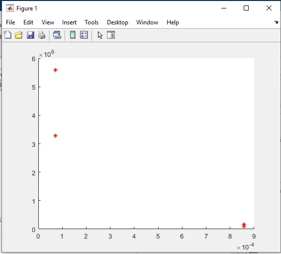
FUNCTION PROGRAM
* After ploting all states we we need plot volume trace for isentropic ,compression , and explain & as we know the volume process it will be straight line
* Plot the curve volume trace we use formula.
* `V = [1+0.5 *(Cr-1).[R+1-COS(theta)-(R^2 -SIN(theta)^2)^(1/2)]]`
* We create the function from this formula as it uses all the parameters and it wil create the trace.
* The function program is:
function [v]= engine_kienamatics(bore,stroke,con_rod,cr,start_crank,end_crank)


a = stroke/2;
R = con_rod/a;

v_s = (pi/4)*bore^2*stroke;
v_c = v_s/(cr-1);

theta = linspace(start_crank,end_crank,100)
term1 = 0.5*(cr-1);
term2 = R +1 - cosd(theta);
term3 = (R^2 - sind(theta).^2).^0.5;
v = (1 + term1*(term2 - term3)).*v_c;


end
* Function command helps us calling any formula or code we need into another.
* [v]= engine_kienamatics(bore,stroke,con_rod,cr,start_crank,end_crank)
* We use the same function in the main function to call function.
* This plot shows us how isentropic curve looks like during compression stroke & expanssion.
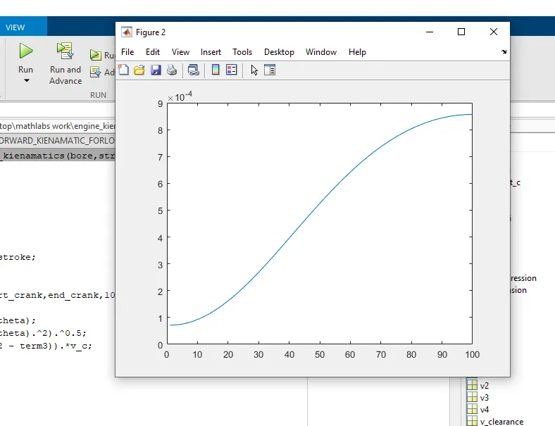
Main Program
* The function is then called and placed in process 1-2 that is isentropic compression and is called v_compression
*The thermal efficiency formulla for the otto cycle is
`E = m.Cv(t3-t2) - (m.Cv(T4-T1))/(m.Cv(t3-t2)`
`E = 1 - ((t4-t1)/(t3-t2))`
`E = 1-(1851.25-500)/(2300-1351)*100`
E = 62.99%
PV-Diagram as a path function- otto cycle
COMMAND

REFERENCES
1 wikipedia
2 Dr. M.K. Muralidhara
3 Dr. B.K. Muralidhara
4 Dr. C.K. Umesh