Curve Fitting
AIM: To perform a curve fitting for a given dataset and to find the best and perfect fit for that particular dataset using Matlab's.
What Is Curve Fitting?
Curve Fitting is a process of constructing a curve which has the closest similarity for the series of data being considered. This method really helps in the mathematical modeling of an experimental or natural process.
Curve Fitting is the process of constructing a curve, or mathematically functions which possess the closest proximity to the real series of data.By curve fitting we can mathematically construct The functional relationship between the observed dataset And parameter values etc. It is highly effective in mathematical modelling of some major processes.
Assume Date a point (11,x2) (x2,x3)..............(xn,yn). And assume the best fit for the set of points will be y=f(x) the criterion Under which the equation of curve will be the Best fit possible as follows: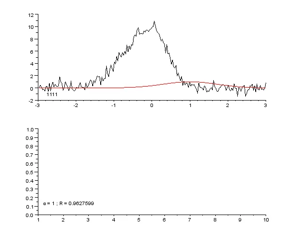
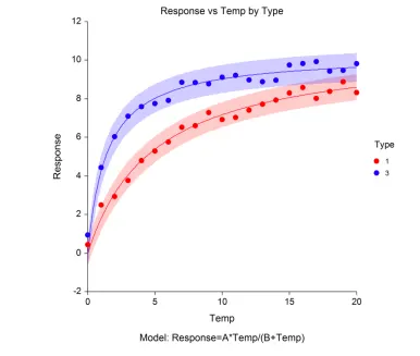
Suppose each of these n points has an individual error (Difference in y-coordinate values )
The error for the general "i" point can be given by the function,
Error = |`y(i)` - value of `f(x)` at `x(i)`| =|`y(i) - f(x(i))`|
To remove the modulus sign, it is effective if we square the error term, when we square the error term and add the errors for all the 'n' points we get,
SSE(sum of squred errors) = `sum_(i=0)^n`ERROR`(i)^2`
assume the proposed equation in nth degree olynomail of the form,
f(x)=`A 1 + A 2 . x + A 3 . x ^2 + ... ... ... ... + A n . x^( n − 1)`
when we differentiate the SSE witheach and every coefficient of the proposed equation f(x). we equate it to zero. we can find the minimaand the value of coefficient
`[ (δ S S E )/(δ A 1) = 0 : (δ S S E)/( δ A 2) = 0 : ..... : (δ S S E )/(δ A 3) = 0 ]`
Upon solving the multiple system of equation we can find the value of all the coefficient.
This method is called Least Square Method and it is mostly commly used technique as long as fitting function is a polynomial
How to choose the best fit:
Upon finding a curve which Satisfies the data points there are four quantities which helps us as major the goodness of fit criteria or how well the equation is representing the data point is there are
The sum of square Due to errors (SSE)
R-Square
Adjust R-square
Root mean square error(RMSE)
R-square:
This quantity that measures how successful the fit is in explaining the variation of the data put another way R-Square is the square of the correlation between the response value and the predicted response value it is also called the Square Of the multiple correlation coefficient and that coefficient of multiple determination
What that means in Laymans terms Is that the higher the value of R-square the better the fit The lower it is the lousier the fit R -square ranges from a value of 0 to1.
0 for the worst possible fit for the dataset.
1 for the best possible fit for the dataset.
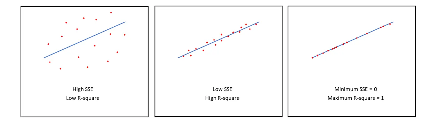
The value of R-Square can be calculated by using formula:
`R^2 = (SSR)/(SST)`
where
SSR→sume of squares of the regression which is basically the square of the differance between the value of fitting function at a given point and the armetic mean of the dataset.
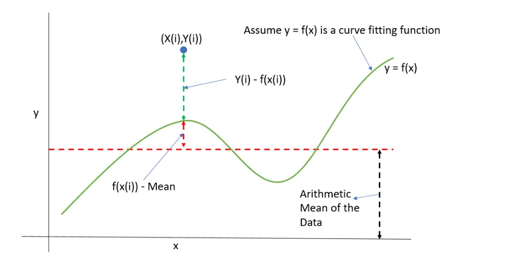
if y=`f(x)` is the fit curve then the SSR is defined as follows:
SSR = `sum_(i=0)^n (f(x(i)) - Mean)^2`
similarly SSE is defined as follows:
SSR= `sum_(i=0)^n (y(i) - f(x(i)))^2`
Now the term SST is given by the summation of SSR and SSE
SST = SSR+SSE;
From here we can calculate the value of `R^2`
`R^2 = (SSR)/(SST)`
Selecting a Preset Model:Over thirty preset models are available. These models provide a variety of curve shapes. Several of the models
were developed for quite different physical processes but yield similar results. We now present examples and
details of several of the preset models available.
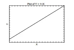
1. Linear: Y=A+BX:This common model is usually fit using standard linear regression techniques. We include it here to allow for
various special forms made by transforming X and Y.
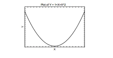
2. Quadratic: Y=A+BX+CX2">Y=A+BX+CX2Y=A+BX+CX2: The quadratic or second-order polynomial model results in the familiar parabola.
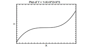
3. Cubic: Y=A+BX+CX2+DX3">Y=A+BX+CX2+DX3Y=A+BX+CX2+DX3: This is the cubic or third-order polynomial model.
Matlab code to fit A inear and cubic polynomial for the cp_data:
%curve fitting a dataset using  linear and cubic polynomial:

clear all
close all
clc


% Entering the data


cp_data = load('data');
temperature=cp_data(:,1);
cp=cp_data(:,2);


% curve fit
%cp =A*t^2 + B*t + C

% finding the coefficient (linear)

[co_efficient,~,mu] = polyfit(temperature,cp,1);

% predicting the cp1
predicted_cp1 = polyval(co_efficient,temperature,[],mu);

%finding the coefficient (cubic)
[co_efficient,~,mu] = polyfit(temperature,cp,3);

%predicting the cp3
predicted_cp3 = polyval(co_efficient,temperature,[],mu);

%compraring the original data and curve fit

plot(temperature,cp,'linewidth',3)
hold on
plot(temperature,predicted_cp1,'linewidth',3,'color','r')
hold on
plot(temperature,predicted_cp3,'linewidth',3,'color','g')
hold off
grid on
legend('orginal dataset','linear curve fit','cubic curve fit')
xlabel('Temperature(k)')
ylabel('specific heat(KJ/K.mol-K)')
title('original data with linear & cubic curve fit')


%R^2 method to find the fitness of the curve
M=mean(cp);
%finding  R^2 for linear
for i= 1:length(cp)
    SSR1=(predicted_cp1(i)-M)^2
    SSE1=(cp(i)-predicted_cp1(i))^2
end
  SST1= SSR1+SSE1;
     R1=SSR1/SST1
%finding R^2 for cubic
for i= 1:length(cp)
    SSR3=(predicted_cp3(i)-M)^2
    SSE3=(cp(i)-predicted_cp3(i))^2
end
SST3=SSR3+SSE3;
Step-wise Explanation Of The Code:
- Firstly we are giving the input data for the program. A file which has the data of the temperature & its corresponding specific heat is taken into the program with the command called 'Load'
- Then the first coulumn is the temperature data and the second coulum is the specific heat data which is inputed into a variable 'temperature' & 'cp' respectively.
- Curve fit is the mathamatical expression.which we can predict the dependent data corresponding to that independent data , for doing this we need to specify a polynomial of any order.
- Then in that polynomial function we have coefficient.we ave to find the coefficient values in order to execute that function for predicting the dataset.
- For linear polynomial.
- cp = A*t +c, here we have to find the coefficient of A.
- For cubic polynomial.
- cp = `A.t^2 + B.t^2 +C.t + D` here we have to find the coefficient of A,B,&C.
- We will use the 'polyfit' command in that we need to specify the dependent variable, independent variable and the order of the polynomial.
- For linear polynomial we give 1.
- For cubic polynomial we give 3.
- Then we need to predict the dataset by using these values of coefficient in a command called 'polyval'.
- By using the coefficient values (A,B,C) and independent data (temperature) into the polyval command.we can actually predict the dependent value (cp).
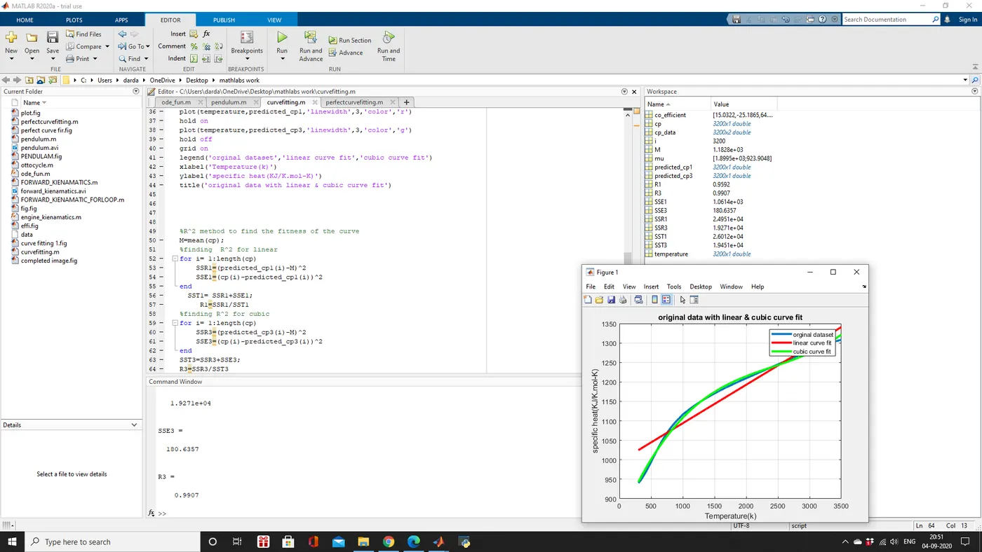
- Then we need to plot the orginal dataset with temperature at x-axis and cp data at y-axis and we are comparing the orginal data and curve fit data that is predicted dataset with linearand cubic curve data.
- now we cn compare the linear and cubic data curve with orginal data curve and figure out which one represents the orginal dataset in a better way.
- Now to find the goodness of the curve fit we are using R-SQUARE Method.
- `R^2 = (SSR)/(SST)`
M=mean(cp)
for i= 1:length(cp)
SSR=(predicted_cp(i)-M)^2
SSE=(cp(i)-predicted_cp(i))^2
end
* Herwe we need to find the mean value of cp that is = (The sum of all cp)/(length of cp).
- To execute the value of `R^2` we are using 'for loop' which repeats the action until the specified condition gets satisfied.
- we are defining the 'i' value to start from 1 and go upto the length of cp.
- SSR is the square of the differance between the predicted cp coressponding to the 'i' value and the mean.
- SSE is the square of the differance between the orginal cp data and the predicted cp data.
- SST is the sum of SSR & SSE, by having all this we can find `R^2` using above formula.
- we do this both linear and cubic polynomials to find the value of R.
- By knowing the value of R we can say the fitness of the predicted curve.
Output for the above program:
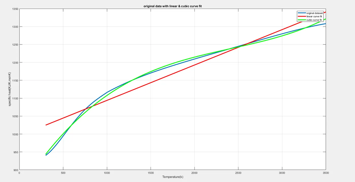
Screenshot Of output:
WORKSPACE:
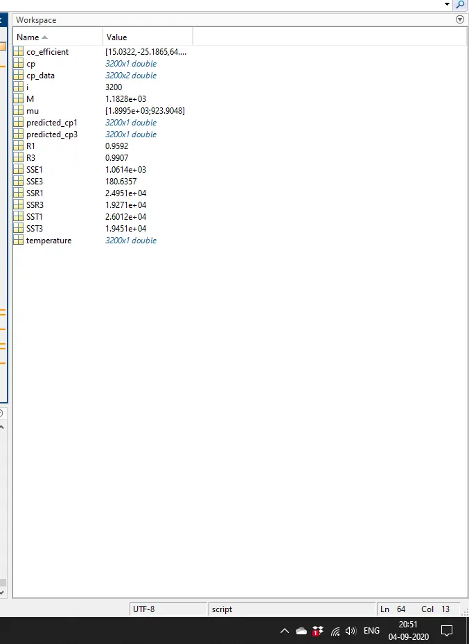
- The workspace shows the value of the linear curve fit R1=0.9592
- The workspace shows the value of the cubic curve fit R3=0.9907
HOW TO FIND THE BEST CURVE:
- The best curve fit should closely represent the original dataset . which degree of the polynomial when used , result `R^2` value more close to 1 that is the best curve fit.
- From the above findings we can say that the cubic curve fit R3 valve is more close to 1 so the cubic curve fit is representing values very close to the orginal dataset.
- The Best curve fit from the above program is the cubic polynomial curve fit which has the `R^2` value ,R3=0.9907.
How TO Improve Fit:
- By using the scaling and centring process we can improve the fit.
- There is another method of spliting the detaset to find the predicted data with the independent variable we can split range from 0 to 5 times and we can use different order of the polynomial for fitting the data at each temperature range.
- Using that process we can improve the fit.
How To Find The Perfect Fit:
- As the Perfect curve fit is yet not done which has the value of `R^2` to be 1. we are doing another coding to make `R^2` value to be 1 so that the perfect cp value matches theorginal cp values.
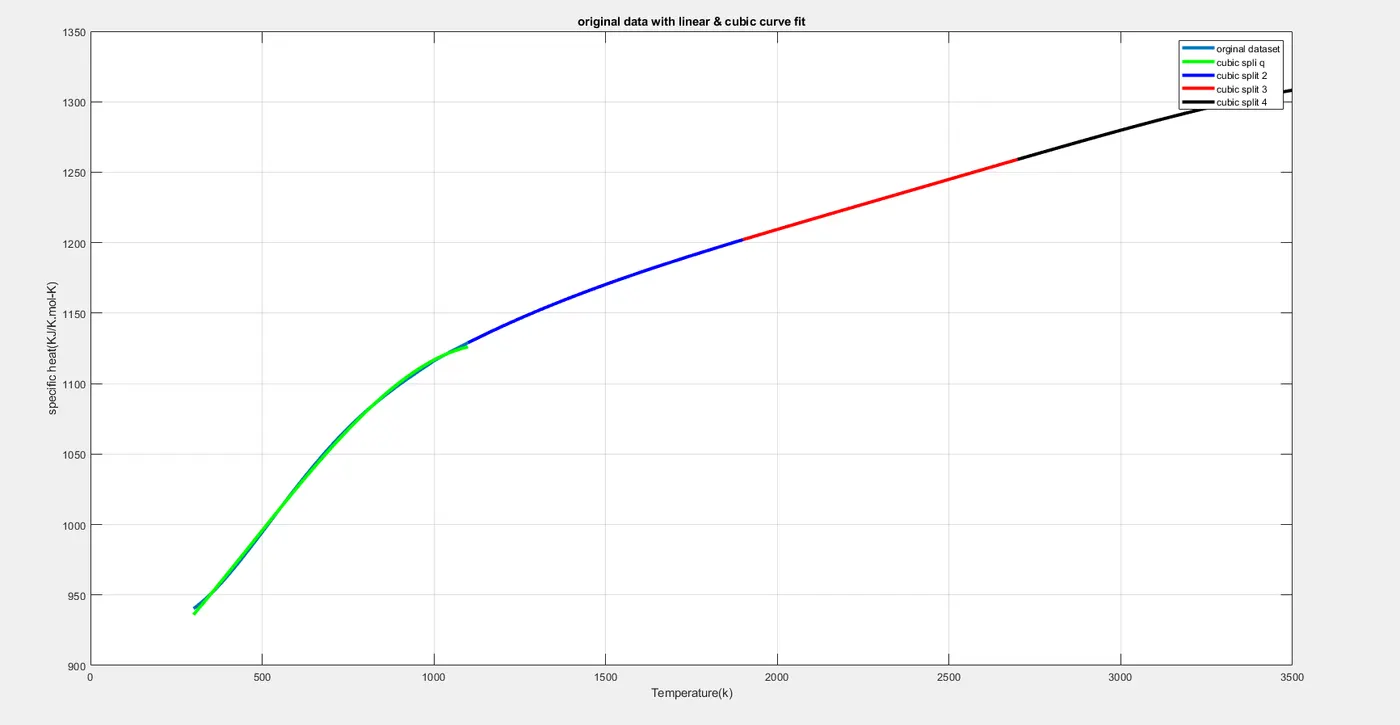
- For doing this we are using the split wise polynomial method, where we split the temperature range equally and will be eecuted the program with different polynomials order at each temperature range to achive the perfect fit for the given dataset so that we may use it for the future prediction of data.
Program To Find The Perfect Curve Fit:
%splitwise method to find perfect fit

clear all
close all
clc

% Entering the data


cp_data = load('data');
temperature=cp_data(:,1);
cp=cp_data(:,2);


%splitting the given data


t1=cp_data(1:800,1);
t2=cp_data(801:1600,1);
t3=cp_data(1601:2400,1);
t4=cp_data(2401:3200,1);
cp1=cp_data(1:800,2);
cp2=cp_data(801:1600,2);
cp3=cp_data(1601:2400,2);
cp4=cp_data(2401:3200,2);

%finding the coefficients off all the temperature range(5th order polynomail)
[co_efficient,~,mu] = polyfit(temperature,cp,5);
predicted_cp = polyval(co_efficient,temperature,[],mu);

%finding the coffiecient in spliwise order(first temperature range)
[co_efficient,~,mu] = polyfit(t1,cp1,3);
predicted_cp1 = polyval(co_efficient,t1,[],mu);

%second temperature range
[co_efficient,~,mu] = polyfit(t2,cp2,3);
predicted_cp2 = polyval(co_efficient,t2,[],mu);

%third temperature range
[co_efficient,~,mu] = polyfit(t3,cp3,3);
predicted_cp3 = polyval(co_efficient,t3,[],mu);


%fourth temperature range
[co_efficient,~,mu] = polyfit(t4,cp4,3);
predicted_cp4 = polyval(co_efficient,t4,[],mu);


%comparing the original  data and curve  fit


plot(temperature,cp,'linewidth',3)
hold on
plot(t1,predicted_cp1,'linewidth',3,'color','g')
hold on
plot(t2,predicted_cp2,'linewidth',3,'color','b')
hold on
plot(t3,predicted_cp3,'linewidth',3,'color','r')
hold on
plot(t4,predicted_cp4,'linewidth',3,'color','k')
hold off
grid on

legend('orginal dataset','cubic spli q','cubic split 2','cubic split 3','cubic split 4')
xlabel('Temperature(k)')
ylabel('specific heat(KJ/K.mol-K)')
title('original data with linear & cubic curve fit')

%R^2 method to find the fitness of the curve
M=mean(cp);
%finding  R^2 for linear
for i= 1:length(cp)
    SSR=(predicted_cp(i)-M)^2
    SSE=(cp(i)-predicted_cp(i))^2
end
  SST= SSR+SSE;
     R=SSR/SST
Output Of The Perfect Curve FIT:
Workspace:
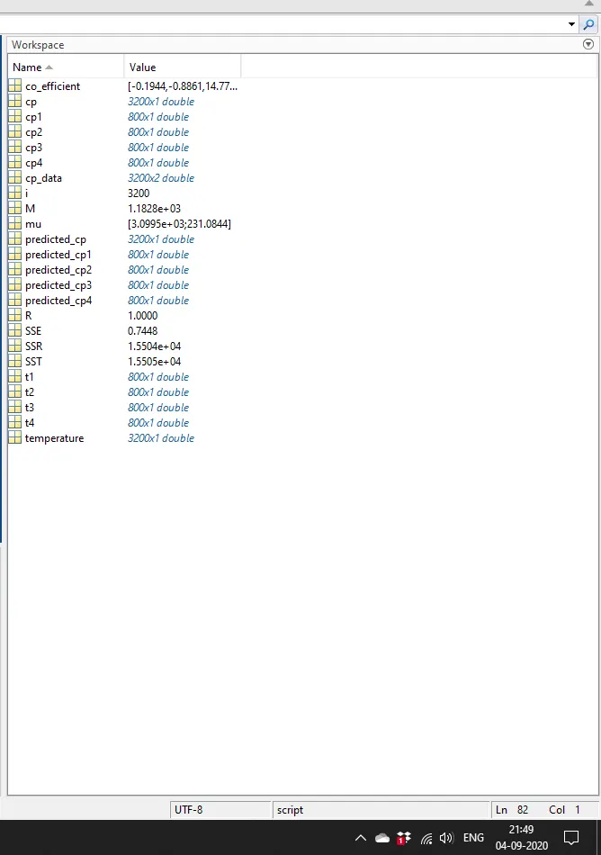
- The value of `R^2` That means the program satisfy the perfect curve fit.
REFERENCE: