AIM:  To create a program in matlab tosolve the second order ODE of the motion of a simple pendulum with damping.

`(d^2theta)/dt^2 +(b/m).(d theta)/dt +(g/l).sintheta = 0`

Objective: To simulate the transient behaviour  of simple pendulum and creating animation of it motion using matlabs.

SIMPLE PENDULUM:

A pendulum is a device that is found in wall clocks. It consists of a weight (bob) suspended from a pivot by a string or a very light rod so that it can swing freely. When displaced to an initial angle and released, the pendulum will swing back and forth with a periodic motion. By applying Newton’s second law of motion for rotational systems, the equation of motion for the pendulum may be obtained.Although the pendulum has a long history, Italian scientist Galileo Galilei was the first to study the properties of pendulums, beginning around 1602.

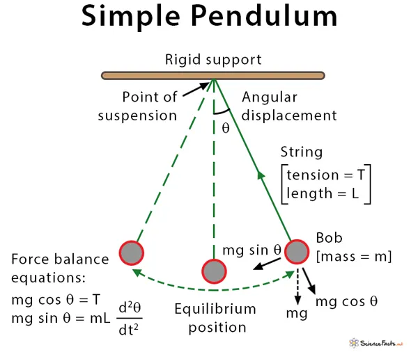
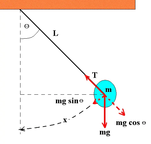
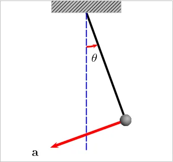
Terms Associated with Simple Pendulum

Length (L): Distance between the point of suspension to the center of the bob

Time period (T): Time taken by the pendulum to finish one full oscillation

Displacement (x): Distance traveled by the pendulum bob from the equilibrium position to one side. The angle described by the pendulum with an imaginary axis at the equilibrium position is called the angular displacement (θ).

The motion of the pendulum is called a simnple harmonic motion and the differential equation which represents the motion of a simple pendulum is:

`(d^2theta)/dt^2 +g/l . sintheta = 0`

where;

g=acceleration due to gravity in `m/s^2`

l=length of the pendulum in 'm'

`theta` =angular displacement

As mention before, real pendulam experience resistive force and hence there osillation die out with time. this effectis called damping the differentail equation for motion of simple pendulum wiith damping.

 `(d^2theta)/dt^2 +(b/m).(d theta)/dt +(g/l).sintheta = 0`

where;

g=acceleration due to gravity in `m/s^2`

l=length of the pendulum in 'm'

`theta` =angular displacement

b=damping coefficient.

Differential equation

In mathematics, a differential equation is an equation that relates one or more functions and their derivatives.^[1] In applications, the functions generally represent physical quantities, the derivatives represent their rates of change, and the differential equation defines a relationship between the two. Such relations are common, therefore differential equations play a prominent role in many disciplines including engineering, physics, etc.

Mainly the study of differential equations consists of the study of their solutions (the set of functions that satisfy each equation), and of the properties of their solutions. Only the simplest differential equations are solvable by explicit formulas; however, many properties of solutions of a given differential equation may be determined without computing them exactly.

Often when a closed-form expression for the solutions is not available, solutions may be approximated numerically using computers. The theory of dynamical systems puts emphasis on qualitative analysis of systems described by differential equations, while many numerical methods have been developed to determine solutions with a given degree of accuracy.

ODE45:

ODE45 is input solver matlab that solves the differentail equation in this case we provide it with two inputs arguments and function which contaims the first order differentail equation

 `(d^2theta)/dt^2 +(b/m).(d theta)/dt +(g/l).sintheta = 0`

The equation is 2nd order differentail equation that solve pendulum motion.

we need breaking down the 2nd order ODE into 1st order ODE. so that ODE45 can solve it.

lets say,

`theta=theta1`

`(d theta)/dt = (d theta)/dt = theta2`    -------------------------------(1)

`(d^2theta)/dt = (d theta1^2)/dt^2 =d/dt ((d theta1)/dt) = d/dt(theta2)`      --------------------------------(2)

we know,

 `(d^2theta)/dt^2 +(b/m).(d theta)/dt +(g/l).sintheta = 0`

`(d^2theta1)/dt^2 +(b/m).(d theta1)/dt +(g/l).sintheta1 = 0`

`(d theta2)/dt +(b/m)(theta) +(g/l).sintheta1 = 0`

`(d theta1)/dt = theta2`     ----------------------------(1st ODE)

`(d theta)/dt = -b/l.theta2 - g/l .sintheta1`

code:

Function to calculate the ODE's

function[dtheta_dt] = ode_fun(t,theta,b,g,l,m)

theta1 = theta(1)
theta2 = theta(2)
dtheta1_dt = theta2;
dtheta2_dt =-(b/m)*theta2-(g/l)*sin(theta1);
dtheta_dt = [dtheta1_dt; dtheta2_dt];
end

Main code

Code to calculate the displacement and velocity with respect to time using ode45 solver and also plotting the  result frame by frame to get an animation t=30 sec.

clear all
close all
 clc
 
 b = 0.05;
 g = 9.81;
 l = 1;
 m = 0.1;
 
 % intail condition
 % intial position 0 of radians, intial velocity 5 rad/s 
 theta_0 = [0;5];  %[displacement,velocity]
 
 % time 
 % time span to simulate the motion 0-30 sec.
 t_span = linspace(0,30,500);
 
 % solve ODE
 % using ode function to obtain results[displacement;velocity]
 [t,result] = ode45(@(t,theta) ode_fun(t,theta,b,g,l,m),t_span, theta_0);
 
 % output plot
 plot(t,result(:,1))
 hold on
 plot(t,result(:,2))
 xlabel('time')
 ylabel('angular displacement and angular velocity')
 grid on
 legend('angular displacement','angular velocity')
 hold off
  
 % plotting pendulum
 figure
 ct=1; %loop counter
 for i = 1:length(t_span)
     x_fixed=0;
     y_fixed=0;
     x_freeend=l*sin(result(i,1));
     y_freeend=-l*cos(result(i,1));
     plot([x_fixed x_freeend],[y_fixed y_freeend],[-0.5 0.5],[0 0],'linewidth',3)
     hold on
     plot(x_freeend,y_freeend,'marker','o','markersize',30,'markerfacecolor','r')
     axis([-1.5 1.5 -1.5 0.5])
     grid on
     pause(0.02)
     M(ct)=getframe(gcf);
     ct=ct+1;
     hold off
 end

movie(M) 
videofile = VideoWriter('pendulum.avi','uncompressed AVI');
open(videofile)
writeVideo(videofile,M)
close(videofile)

 CODE FOR CREATING THE MOVIE:

movie(M) 
videofile = VideoWriter('pendulum.avi','uncompressed AVI');
open(videofile)
writeVideo(videofile,M)
close(videofile)

Step 1:  

* clear all, close all & clc . used to clear all the cvariable in the workspace.

* To close all the figures and plots.

* clear the command the window all pervious notations and values respectively.

Step 2: Declearing the input parameters

* here the required input parameter are deceleard like length of the string, mass of the bob, damping coefficient and the acc. duee to gravity

Step 3: Initial conditions and time period

* here we are dfinng the initial condition like angular dispacement & angular velocity in the form of an array into a new variable called theta_0 then the time period of the osscillation is declared with the help of linspace command  from 0 to 30 with 500  points and assigning it to variable called time span.

Step 4:  Calculating the function ODE45.

* In this step we are solving the ode equation with the help of inbuilt ode command in the matlabs 

% solving ode

[t,result] = ode45(@(t,theta) ode_fun(t,theta,b,g,l,m),t_span, theta_0);

here we are deffining ode45 is the function of t and theta because 't' and 'theta' is the oly dependent and independent variable of the ode system then  we are calling our function which has input parameter variable followed by the time_span array and theta_0(initial codition)

Step 5: Plotting  graph 

* here we are plotting the graph which shows the angular  velocity and angular displacement  with respect to the time period of osscillation we can observed  the changes in the graph by channging the damping co-efficient also.

Step 6: Creating animation with the for loop.

* here in for loop we are declaring the value with the range operator to length of the result value 1.which is nothing but the angular displacement value

* then we are assigning into new variablecaleed(i).

* next process is to give the coordinates value for the string where the ball is hangging x0,y0 & x1,y1 are the variable which stores the value for string .

Step 7: Plotting the figure under the for loop

* durring plotting under the for loop the ball is plotted at the end  of the string with the help of marker and markersize and face color is also declared.

Step 8: 

* finally we create the video file  with the help of getframe,loop counter , videowrite and open video ,closevideo command. 

PLOTTING FIGURE:

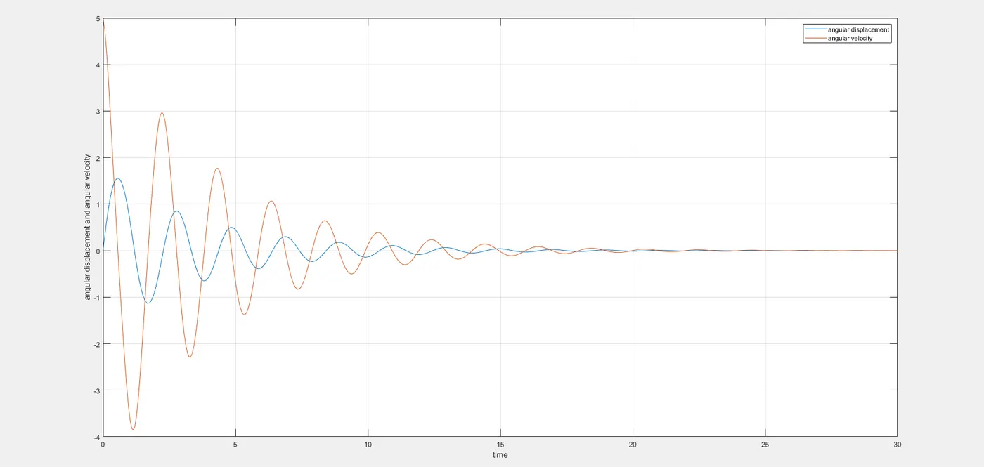
The above graph of angular velocity and angular displacement with respect to 30secs time, shows that the displacement and velocity reduce with the time due to damping coefficient..

If the damping coefficient value is set to 0. it will give never ending motion theoretically in practical coding the program skips the value of b(damping coefficient) and runs  the program for the define value of the time.

ANIMATION:

https://youtu.be/ZIFFc7BaGxU

ERRORS:

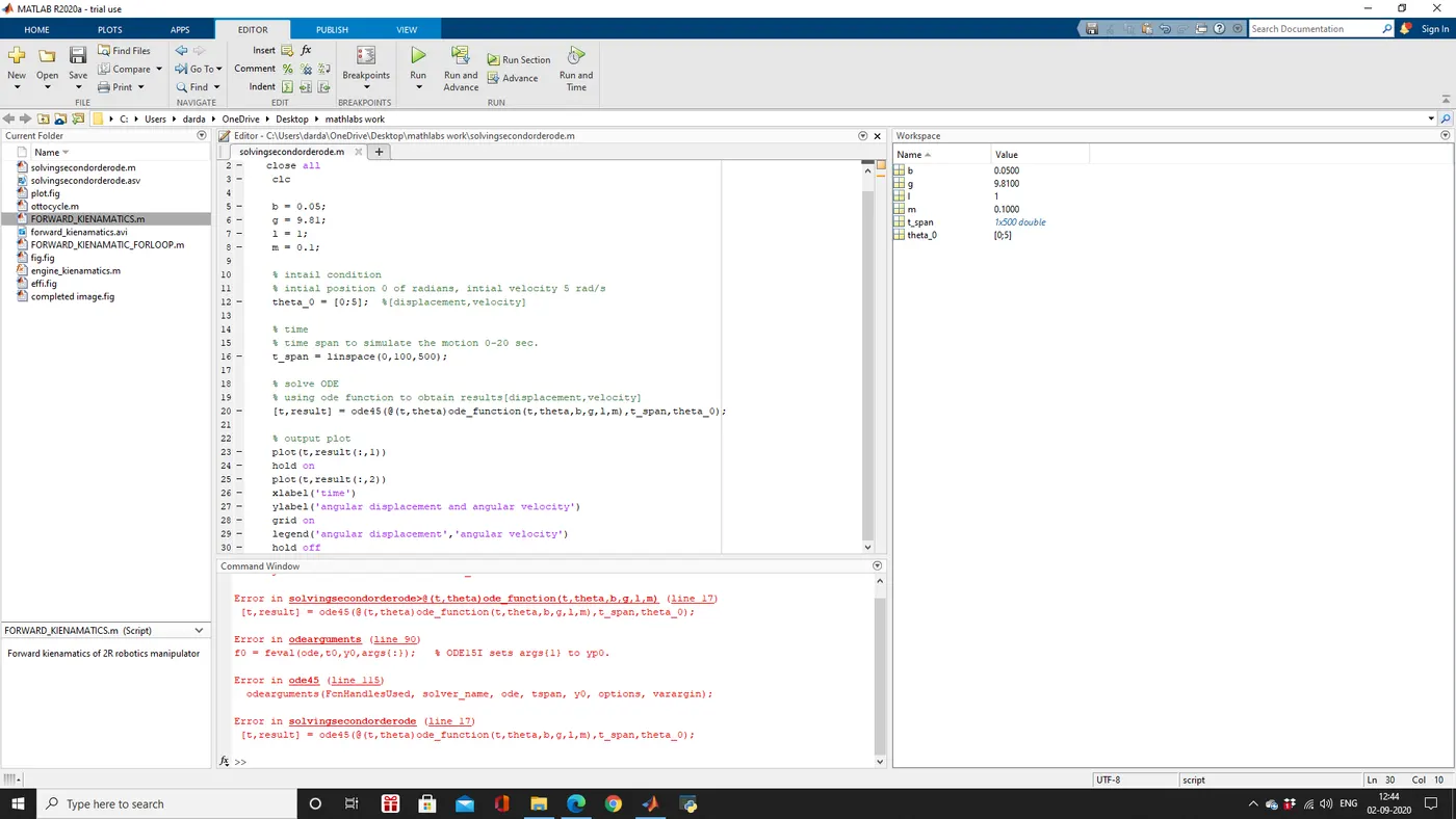
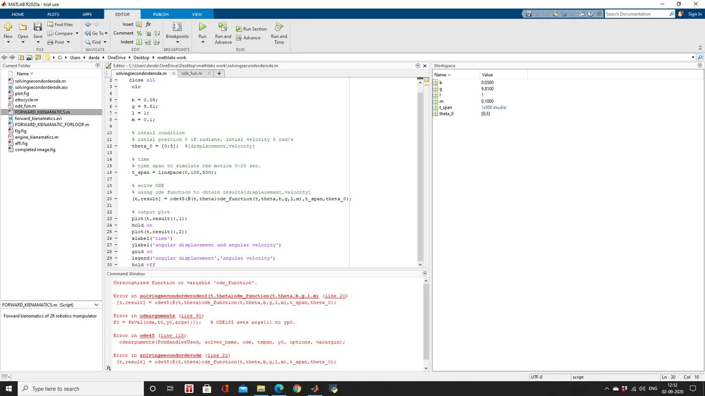
The error i was getting i was writing ode_function but i have to write ode_fun

  REFRENCE:

Wikipedia