Week 4 - Genetic Algorithm
Introduction: In this project, I try to understand the concept of the genetic algorithm by referring to various sources. I wrote a code in MATLAB to optimize the stalagmite function and find the global maxima of the function and I explain the concept of genetic algorithm and also explain the syntax for ga in MATLAB.
What is a Genetic Algorithm?
A genetic algorithm (GA) is a method for solving both constrained and unconstrained optimization problems based on a natural selection process that mimics biological evolution. The algorithm repeatedly modifies a population of individual solutions. At each step, the genetic algorithm randomly selects individuals from the current population and uses them as parents to produce the children for the next generation. Over successive generations, the population "evolves" toward an optimal solution.
You can apply the genetic algorithm to solve problems that are not well suited for standard optimization algorithms, including problems in which the objective function is discontinuous, nondifferentiable, stochastic, or highly nonlinear.
It generates a population of points at each iteration and the best point in the population approaches an optimal solution. It elects the next population by computation which uses random number generators.
How does the Genetic Algorithm work?
The following outline summarizes how the genetic algorithm works:
-
The algorithm begins by creating a random initial population.
-
The algorithm then creates a sequence of new populations. At each step, the algorithm uses the individuals in the current generation to create the next population. To create the new population, the algorithm performs the following steps:
-
Scores each member of the current population by computing its fitness value. These values are called the raw fitness scores.
-
Scales the raw fitness scores to convert them into a more usable range of values. These scaled values are called expectation values.
-
Selects members, called parents, based on their expectation.
-
Some of the individuals in the current population that have lower fitness are chosen as elite. These elite individuals are passed to the next population.
-
Produces children from the parents. Children are produced either by making random changes to a single parent—mutation—or by combining the vector entries of a pair of parents—crossover.
-
Replaces the current population with the children to form the next generation.
-
-
The algorithm stops when one of the stopping criteria is met.
Syntax of Genetic algorithm:
x = ga(fun,nvars)x, to the objective function, fun. nvars is the dimension (number of design variables) of fun.
x = ga(fun,nvars,A,b)x to fun, subject to the linear inequalities A*x ≤ b. ga evaluates the matrix product A*x as if x is transposed (A*x').
x = ga(fun,nvars,A,b,Aeq,beq)x to fun, subject to the linear equalities Aeq*x = beq and A*x ≤ b. (Set A=[] and b=[] if no linear inequalities exist.) ga evaluates the matrix product Aeq*x as if x is transposed (Aeq*x').
x = ga(fun,nvars,A,b,Aeq,beq,lb,ub)x, so that a solution is found in the range lb ≤ x ≤ ub. (Set Aeq=[] and beq=[] if no linear equalities exist.)
x = ga(fun,nvars,A,b,Aeq,beq,lb,ub,nonlcon)nonlcon. The function nonlcon accepts x and returns vectors C and Ceq, representing the nonlinear inequalities and equalities respectively. ga minimizes the fun such that C(x) ≤ 0 and Ceq(x) = 0. (Set lb=[] and ub=[] if no bounds exist.)
x = ga(fun,nvars,A,b,Aeq,beq,lb,ub,nonlcon,options)options. (Set nonlcon=[] if no nonlinear constraints exist.) Create options using optimoptions.
for example,
options = optimoptions('ga','ConstraintTolerance',1e-6,'populationsize',250);
x = ga(fun,nvars,A,b,[],[],lb,ub,nonlcon,IntCon)x = ga(fun,nvars,A,b,[],[],lb,ub,nonlcon,IntCon,options)IntCon take integer values.
x = ga(problem)problem, where problem is a structure.
[x,fval,exitflag,output,population,scores] = ga(___) also returns a matrix population, whose rows are the final population, and a vector scores, the scores of the final population.clear all
close all
clc
%inputs
x=linspace(0,0.6,150);
y=linspace(0,0.6,150);
%converting into 2d mesh
[xx, yy]= meshgrid(x,y);
%creating a stalagmite function output using stalagmite() function
for i=1:length(xx)
for j=1:length(yy)
input_vector(1)=xx(i,j);
input_vector(2)=yy(i,j);
f(i,j)=stalagmite(input_vector);
end
end
%Plotting the function using surfc
surfc(xx,yy,f)
shading interp
title('Stalagmite Function optimization Basic')
%genetic algorithm optimization
[input,fval]=ga(@stalagmite,2)
%stalagmite function
function [f]=stalagmite(input_vector)
x=input_vector(1);
y=input_vector(2);
% Formula of Stalagmite Function
term1=(sin((5.1*pi*x)+0.5))^6;
term2=(sin((5.1*pi*y)+0.5))^6;
term3=exp(-4*log(2)*((x-0.0667)^2)/0.64);
term4=exp(-4*log(2)*((y-0.0667)^2)/0.64);
f=-(term1*term2*term3*term4);
end
Explanation of code: Here I converted the x and y input into 2d mesh. I created a variable f in which I stored the outputs from the stalagmite function. Using the surfc command I created a 3D plot of the function and using the ga(Genetic Algorithm) function I input the stalagmite function and the number of variable(x and y). In the stalagmite function code I just wrote out the formula of the stalagmite and passed the value as negatiive because the ga function only calculates the minima.
Output Explanation: The ga function is all over the place and has only one iteration, thus, it calculates the minima differently every time we execute the program.
To make sure that ga only gives a single output every time we use the following program:
Code 2:
clear all
close all
clc
%input
x=linspace(0,0.6,100);
y=linspace(0,0.6,100);
%number of times ga to be run
num_cases=50;
%calling the get_staalagmite function for 2d mesh
f=get_stalagmite(x,y);
%calculating ga and also the time taken by it
tic
for i=1:num_cases
[input,f_opt(i)]=ga(@stalagmite,2);
x_opt(i)=input(1);
y_opt(i)=input(2);
end
time1=toc
%dividing the figure into two parts
figure(1)
%plotting the stalagmite function
subplot(2,1,1)
xlabel('X values')
ylabel('Y values')
zlabel('Optimum value')
surfc(x,y,f)
hold on
title('Unbounded GA with output plot of ga values')
shading interp
%plotting the output x and y and output optimum value in the first row
plot3(x_opt,y_opt,f_opt,'marker','o','markersize',5,'markerfacecolor','r')
%plotting the optimum value w.r.t. number of iterations
subplot(2,1,2)
plot(f_opt)
title('Output value w.r.t. iterations')
xlabel('Iterations')
ylabel('GA Output values')
%Case 2:setting of lower and upper bounds on the design variables
tic
for i=1:num_cases
[input,f_opt(i)]=ga(@stalagmite,2,[],[],[],[],[0;0],[0.6;0.6]);
x_opt(i)=input(1);
y_opt(i)=input(2);
end
time2=toc
figure(2)
%dividing the figure into 2 rows again
subplot(2,1,1)
surfc(x,y,f)
xlabel('X values')
ylabel('Y values')
zlabel('Optimum value')
hold on
title('Unbounded GA with output plot of ga values')
shading interp
%checking the output in the stalagmite function
plot3(x_opt,y_opt,f_opt,'marker','o','markersize',5,'markerfacecolor','r')
%plotting output wrt iterations
subplot(2,1,2)
plot(f_opt)
title('Output value w.r.t. iterations')
xlabel('Iterations')
ylabel('GA Output values')
xlabel('Iterations')
ylabel('GA Output values')
xlabel('Iterations')
ylabel('GA Output values')
%Case 3: Setting the population size
%setting the population size to 250
options=optimoptions('ga','populationsize',300)
tic
for i=1:num_cases
[input,f_opt(i)]=ga(@stalagmite,2,[],[],[],[],[0;0],[0.6;0.6],[],[],options);
x_opt(i)=input(1);
y_opt(i)=input(2);
end
time_3=toc
figure(3)
subplot(2,1,1)
hold on
surfc(x,y,f)
xlabel('X values')
ylabel('Y values')
zlabel('Optimum value')
title('Unbounded GA with output plot of ga values')
shading interp
plot3(x_opt,y_opt,f_opt,'marker','o','markersize',5,'markerfacecolor','r')
subplot(2,1,2)
plot(f_opt)
title('Output value w.r.t. iterations')
xlabel('Iterations')
ylabel('GA Output values')
%stalagmite function
function [f]=stalagmite(input_vector)
%taking the input vector values into x and y
x=input_vector(1);
y=input_vector(2);
% Formula of Stalagmite Function
term1=(sin((5.1*pi*x)+0.5))^6;
term2=(sin((5.1*pi*y)+0.5))^6;
term3=exp(-4*log(2)*((x-0.0667)^2)/0.64);
term4=exp(-4*log(2)*((y-0.0667)^2)/0.64);
f=-(term1*term2*term3*term4);end
%get_stalagmite function to create 2d mesh
function [f]=get_stalagmite(x,y)
%creating 2d mesh
[xx, yy]= meshgrid(x,y);
%getting values into f of stalagmite function
for i=1:length(xx)
for j=1:length(yy)
input_vector(1)=xx(i,j);
input_vector(2)=yy(i,j);
f(i,j)=stalagmite(input_vector);
end
end
end
Explanation of the code:
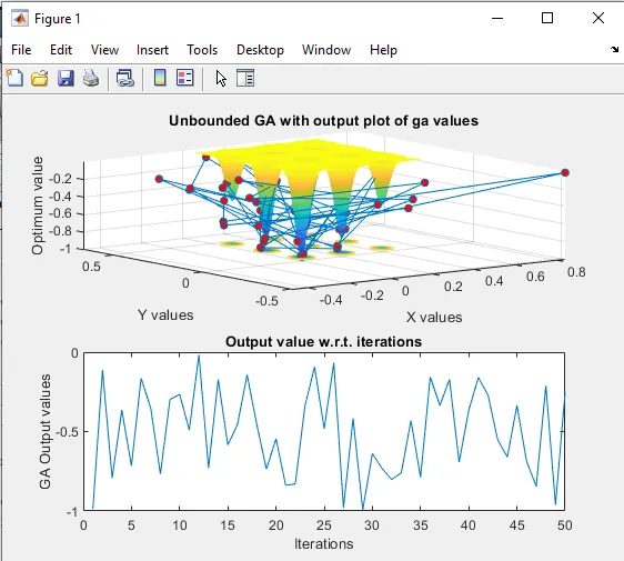
In this code, I called the get_stalagmite function to put the stalagmite function data into the variable f. I have taken number of iterations to be 50(num_cases). In the first part, I ran the ga function 50 times and then plotted the values of the output of ga in the stalagmite function using 'hold on'. Using subplot i divided the figure(1) into two rows and in the second row I plotted the output of the ga function w.r.t time. I calculated the time taken by ga using the tic and toc function in Matlab.
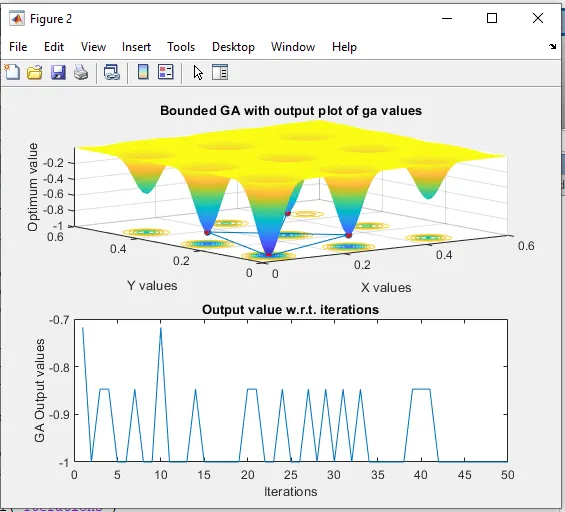
For the second part, since, ga was taking values from all over the place i.e without any bounds, I added the lower and upper bounds using the ga function syntax as mentioned earlier. I calculated the time taken by ga to complete this same as part 1. Similar to the first part I plotted the output into stalagmite function and also the f_opt w.r.t. iterations
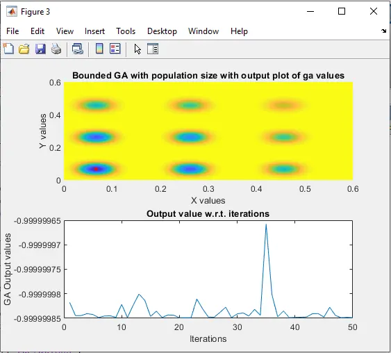
For the 3rd part, I increased the population size to get the optimum value accurately to find the global minima(maxima for us) and the x and y coordinates of when that occurs in the stalagmite function. I did that by again following the ga syntax and the optimoptions command to make the population size of 300. More the size of the population the more the accuracy of the output. However, the tme taken by ga to calculate the global minima increases with the population size.
Output Explanation:
Why did I have to make improvements to part 1 and even part 2?
In the first part, from the figure(1) it is clear that the ga function is calculating the minima all over the place and the 2nd row also shows that the output value calculated by ga is varying very much. Thus, this data is of no use.
To remove this problem I added lower and upper bounds and this improved the output by a good margin and the ga was able to cut down the global minima to 3 places which is still good but no use. Also, the output variation w.r.t. iterations decreased but still needed a bit of narrowing.
Then in the 3rd part, I increased the population size to 300 using the ga syntax and optimoptions function. This made the ga narrow down the global minima(maxima for us) to a specific point and narrowed the variation of output value w.r.t. iterations. Now, this data is very useful to perform optimization. This does have a drawback w.r.t computing time.
Case 1:
Case 2:
Case 3:
Drawbacks
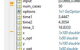
I calculated the time taken by ga to calculate and it increases with the number of conditions.
A very large time is taken when compared part1 time with part 3. This time increases with the size of the population and other constraints.
Errors I faced during the program:
Error1: I forgot to put (i,j) for each value of i and j in the for loop in the get_stalagmite function. It was not returning the proper value of f. I corrected this error by checking and adding f(i,j).
References:
https://in.mathworks.com/help/gads/ga.html#mw_a9a9e523-4242-481e-b6b9-acbe194a2432
https://in.mathworks.com/discovery/genetic-algorithm.html
https://skill-lync.com/knowledgebase/genetic-algorithm-explained