Week 3 - Solving second order ODEs
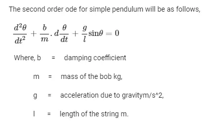
Introduction: The objective of the project is to write a program that solves the following ODE. This ODE represents the equation of motion of a simple pendulum with damping.
Code:
clear all
close all
clc
%solving a ODE
%initially
b=0.05; %damping factor
l=1; %length of the pendulum(m)
m=0.1; %mass of the bob(kg)
g=9.81; %acceleration due to gravity (m/s^2)
%initial conditions at time=0 w=5 rad/sec
theta_0 = [0;5];
%time span
t_span = linspace(0,20,500);
ct=1;
%solving the ODE and calling the function ode_func
[t,results]= ode45(@(t,theta) ode_func(t,theta,b,g,l,m),t_span, theta_0);
%plotting the velocity and displacement change w.r.t. time
plot(t,results(:,1),'color','b')
hold on
plot(t,results(:,2),'color','r')
xlabel('Time')
ylabel('Plot')
legend('Displacement','Velocity')
title('Angular Velocity and Displacement w.r.t. time')
%tracing the movement of pendulum
theta_p= results(:,1);
for i=1:length(theta_p)
THETA=theta_p(i);
x1=0;
y1=0;
x2=l*sin(THETA);
y2=-l*cos(THETA);
figure(2)
%each frame of pendulum in time to trace the movement of pendulum
plot([x1 x2], [y1 y2],'o- ','MarkerIndices',2*l,'MarkerSize',20,'MarkerFaceColor','r','MarkerEdgeColor','r','linewidth',4)
hold on
%plotting the beam to which pendulum is hanging
line([-0.5 0.5],[0 0])
line([-0.5 0.5],[0.05 0.05])
line([-0.5 0.5],[0.1 0.1])
line([-0.5 0.5],[0.15 0.15])
line([-0.5 0.5],[0.2 0.2])
line([-0.5 0.5],[0.25 0.25])
line([-0.5 0.5],[0.3 0.3])
line([0.45 0.45],[0 0.3])
line([0.4 0.4],[0 0.3])
line([0.3 0.3],[0 0.3])
line([0.2 0.2],[0 0.3])
line([-0.45 -0.45],[0 0.3])
line([-0.4 -0.4],[0 0.3])
line([-0.3 -0.3],[0 0.3])
line([-0.2 -0.2],[0 0.3])
line([-0.1 -0.1],[0 0.3])
line([0.1 0.1],[0 0.3])
hold off
title('Movement of a damped Pendulum')
set(gca,'XColor', 'none','YColor','none') %removing the axis from output
axis([-2 2 -2 2]) %setting axis
A(ct)=getframe(gcf); % capturing frame for each ct value and storing in A
ct=ct+1;
end
movie(A)
videofile2=VideoWriter('Pendulum_anime','Uncompressed AVI');
open(videofile2)
writeVideo(videofile2,A)
close(videofile2)
function code:
function [V]= ode_func(t,theta,b,g,l,m)
theta1 = theta(1);
theta2 = theta(2);
dtheta1_dt = theta2;
dtheta2_dt= (-b/m)*theta2 - (g/l)*sin(theta1);
V = [dtheta1_dt ; dtheta2_dt];
end
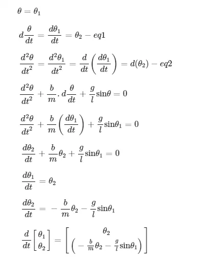
Explanation of the code: I took the input values like mass of the bob, acceleration due to gravity, time span, and the initial conditions. I divided the 0-20s time interval into 500 equally spaced values using the linspace function. To solve the differential equation, I used the ode45 function which solves first-order differential equations. Hence I converted the second-order differential equation into two first-order equations to get the output as the angular displacement and angular velocity.
How does ode45 work?
Ode45 is a function in Matlab that solves ordinary or partial differential equations using a numerical method. The numerical method in question here is the 4th order Runge Kutta method.
To solve an ODE, we have to integrate and solve for the variable. Assuming we have an ode du, we would solve for u by integrating du provided some limits of integration. However, rather than direct integration, we can use a numerical solver, by discretizing the equation, that is, we convert the ODE into a linear equation and then solve this equation to approximate the solution.
I gave the initial conditions and the time_span(for integration in time-step) to the ode45 function. I used the anonymous (@) function for t and theta. To convert and give the differential equation function to ode45. I substituted the theta values into theta1 and theta2 for converting into a first-order differential equation using this technique;
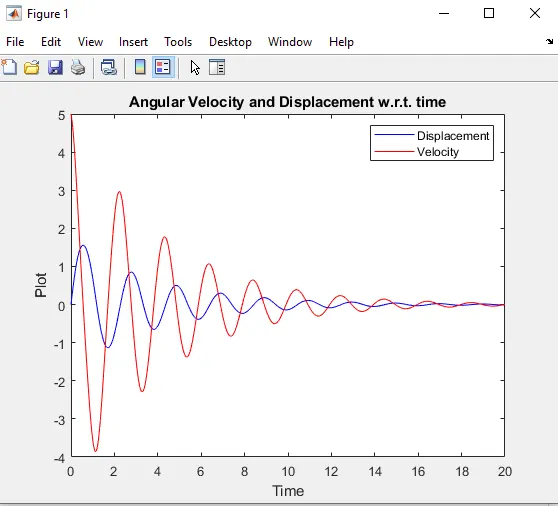
After getting the solution of the differential equation for 0-20 seconds for all 500 parts of time. I plotted the variation of velocity and displacement with respect to time.
To get the animation of the pendulum I took the angular displacement values into theta_p. Using the for loop, I plotted each position of the pendulum in time, i used getframe(gcf) to create the movement. I captured all the frames into variable A and made a movie of it and saved it as an Uncompressed AVI file. To plot the beam, I used 'hold on' and 'hold off' command to plot lines to resemble the beam from which the pendulum is hanging.
Output:
Graph:
Animation picture:
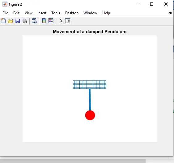
Explanation of the Output: The graph shows the initial displacement and velocity of the pendulum(0 and 5 rad/s). Since the pendulum is damped, the velocity and displacement decrease in the 20-second time span. This is also clear in the output animation video, where initially, the pendulum is at 0 position with 5rad/sec velocity, and the displacement and velocity decrease with time due to the damping factor.
The error I faced during this project: The main error I faced was due to the wrong placement of the hold on command to plot the beam to which the pendulum is hanging. I used it before the plotting of the main pendulum thinking it will work, but in the error picture, it is clear that I was not getting all plot frames with time but all the positions were getting displayed together. I corrected this error by placing the hold on command right before plotting the lines for beam and used hold off command right after I completed the lines for the beam.
References:
https://skill-lync.freshdesk.com/support/solutions/articles/43000580976-understanding-ode45
https://skill-lync.freshdesk.com/support/solutions/articles/43000580974