The Rankine cycle is an idealized thermodynamic cycle of a heat engine that converts heat into mechanical work while undergoing a phase change. It is an idealized cycle in which friction losses in each of the four components are neglected. The heat is supplied externally to a closed loop, which usually uses water as the working fluid.

1.) Boiler for generating steam at constant pressure

2.) A turbine or engine in which steam will expand isentropically and work is done.

3.) A condenser in which heat is removed from the exhaust steam and it is completely converted into the water at constant pressure.

4.) A pump raises the pressure of liquid water to boiler pressure and pumps it into the boiler for converting into steam.

Turbine (1-2): Superheated steam enters into the Turbine and expands isentropically resulting in the production of work. The shaft of the turbine is connected to the generator. This results in the production of electricity i.e Mechanical energy gets converted into electric energy. Work produced by the turbine,

`W_T = m(h_1 -h_2) K`

Condenser (2-3): The expanded vapor is then passed through a condenser, where it gets condensed and converts into liquid again. This liquid is again pumped to the boiler.

`Q_r = m(h_2 - h_3) K`

Pump (3-4): The water enters into the pump in a saturated state. Then the liquid is compressed isentropically until it meets the boiler pressure. Work done by the pump is,

`W_P = m(h_3 -h_4) K`

Boiler (4-1): The water enters into the boiler as compressed and leaves as superheated from the boiler. Thus the phase changes from liquid to vapor. The heat supplied by the boiler is

`Q_b = m(h_1 - h_4) K`

Here we take mass flow rate m = 1 for this code.

The efficiency of the Steam Cycle is given by

`eta = frac{W_n}{Q_1} = frac{W_T-W_P}{Q_1}`

Applying the Steady Flow Energy Equation (SFEE) to all the process, neglecting the Friction losses and changs in Kinetic & Potential Energy,

Q1=h1-h4 @Boiler

Wt=h1-h2 @Turbine

Q2=h2-h3 @Condenser

Wp=h4-h3 @Pump

The Capacity of the Steam Plant is often expressed interms of Steam Rate (SR) or Specific Steam Consumption (SSC)

`S.S.C. = 3600/W_n frac{kg}{kWh}`

Back Work Ratio:

The fraction of the work produced by the turbine that is consumed by the compressor.

Net work output :

w_{net ,out} = w_{turbine, out} - w_{pump, in}

Methods to increase the efficiency of the Rankine cycle

Basic idea: Increase the average temperature at which heat is transferred to the working fluid in the boiler, or decrease the average temperature at which heat is rejected from the working fluid in the condenser.

1. Lowering the condenser Pressure:-

Lowering the operating pressure of the condenser lowers the temperature at which heat is rejected. The overall effect of lowering the condenser pressure is an increase in the thermal efficiency of the cycle.

2. Superheating the steam to high temperatures:-

The average temperature at which heat is added to the steam can be increased without increasing the boiler pressure by superheating the steam to high temperatures.

Superheating the steam to higher temperatures has another very desirable effect: It decreases the moisture content of the steam at the turbine exit.

3. Increasing the Boiler pressure:-

Increasing the operating pressure of the boiler automatically raises the temperature at which boiling takes place.

This raises the average temperature at which heat is added to the steam and thus raises the thermal efficiency of the cycle.

Required Inputs:

Turbine Inlet temperature = 400° C

Turbine Inlet Pressure = 30 bars

Turbine Outlet Pressure = 0.05 bars = Condenser Inlet Pressure

close all
clear all
clc

% Printing the Process 
fprintf('%45s','Rankine Cycle Simulator')
fprintf('\n\n')
fprintf('1-2 Isobaric heat Transfer\n')
fprintf('2-3 Isentropic Expansion\n')
fprintf('3-4 Isobaric heat Rejection\n')
fprintf('4-1 Isentropic Compression\n')

%Enter Inputs
p1 = input('Enter the Pressure at the Turbine Inlet (in bar):');
T1 = input('Enter the Temperature at the Turbineinlet (in Degree Celcius):');
p2 = input('Enter the Pressure at the Condensor (in bar):');

%Calculate each state point values at state point 1
h1 = XSteam('h_pt',p1,T1);
s1 = XSteam('s_pt',p1,T1);

%state point 2
s2=s1;
sf2 = XSteam('sL_p',p2);
sg2 = XSteam('sV_p',p2);
hf2 = XSteam('hL_p',p2);
hg2 = XSteam('hV_p',p2);

%dryness at state point 2
if (s2<=sg2)
    x2 = (s2-sf2)/(sg2-sf2);
else
    x2=1;
end
h2=hf2 +(x2*(hg2-hf2));
            
T2=XSteam('T_hs',h2,s2);

%state point 3
T3=T2;
p3= p2;
s3=XSteam('sL_T',T3);
h3=XSteam('hL_T',T3);
v3 = XSteam('vL_p',p2);

%state point 4
p4 =p1;
s4= s3;
Cp4 = XSteam('Cp_ps',p4,s4);
Cv4 = XSteam('Cv_ps',p4,s4);
gamma = Cp4/Cv4;
r = (gamma - 1)/gamma;
T4 = T3 *(p4/p3)^r;

%Calculate other output values.
% Turbine Work
Wt = h1-h2;       
% Pump Work
Wp = v3*(p1-p2)*100;
h4 = Wp + h3;
% Net Work unit in kj/kg
W_net = Wt-Wp;       
q_in = h1 - h4;  %heat suppied
%heat rejected in condenser
q_out=h2-h3;

%Efficiency
n = (W_net/q_in)*100;
steam_rate = 3600/(Wt - Wp);%Steam rate per second

%back work ratio wp/wt
bwr= Wp/Wt;

%state point 5 and 6 which help in plotting
T5=XSteam('Tsat_p',p1);
T6=T5;s5=XSteam('sL_p',p1);
s6=XSteam('sV_p',p1);
h5=XSteam('hL_p',p1);
h6=XSteam('hV_p',p1);


%print all state poont values to show.
%Results output
fprintf('\n \n \n')
fprintf('%40s \n \n','RESULTS');
fprintf('%10s %54s \n','At State Point 1','At State Point 2');
fprintf('%s %.2f%s %44s %.2f%s \n','P1:',p1,' bar','P2:',p2,' bar');
fprintf('%s %.2f%s %35s %.2f%s \n','T1:',T1,' Deg Celcius','T2:',T2,' Deg Celcius');
fprintf('%s %.2f%s %40s %.2f%s \n','H1:',h1,' KJ/kg','H2:',h2,' KJ/kg');
fprintf('%s %.2f%s %42s %.2f%s \n','S1:',s1,' KJ/kgK','S2:',s2,' KJ/kgK');
fprintf('%58s %.2f \n \n','X2:',x2);
fprintf('%10s %54s \n','At State Point 3','At State Point 4');
fprintf('%s %.2f%s %45s %.2f%s \n','P3:',p3,' bar','P4:',p4,' bar');
fprintf('%s %.2f%s %35s %.2f%s \n','T3:',T3,' Deg Celcius','T4:',T4,' Deg Celcius');
fprintf('%s %.2f%s %41s %.2f%s \n','H3:',h3,' KJ/kg','H4:',h4,' KJ/kg');
fprintf('%s %.2f%s %42s %.2f%s \n \n','S3:',s3,' KJ/kgK','S4:',s4,' KJ/kgK');
fprintf('%40s %.2f %s \n','Work output by Turbine(Wt): ',Wt,' KJ/kg');
fprintf('%40s %.2f %s \n','Work input by Pump(Wp): ',Wp,' KJ/kg');
fprintf('%40s %.2f %s \n','Net Work(Wnet): ',W_net,' KJ/kg');
fprintf('%40s %.2f %s \n','Thermodynamic Efficiency(Ntherm): ',n,'Percent');
fprintf('%40s %.2f %s \n','Heat input in Boiler: ',q_in,' KJ/kg');
fprintf('%40s %.2f %s \n','Heat rejected in condenser: ',q_out,' KJ/kg');
fprintf('%40s %.4f %s \n','Back Work ratio: ',bwr);
fprintf('\n')
fprintf('%40s %.2f %s \n','S.S.C.: ',p3,' Kg/kWh');


%plot T-S Diagram
figure(1)
T_rankine = linspace(T5,T1,5000);
for i = 1:length(T_rankine)
    s_rankine(i) = XSteam('s_pT',p1,T_rankine(i));
end
plot([s1 s2 s3 s4 s5 s6 s_rankine],[T1 T2 T3 T4 T5 T6 T_rankine],'linewidth',1.5);
hold on
T_curve = linspace(1,400,500);
for i=1:length(T_curve)
    s_l(i) = XSteam('sL_T',T_curve(i));
    s_v(i) = XSteam('sV_T',T_curve(i));
    h_l(i) = XSteam('hL_T',T_curve(i));
    h_v(i) = XSteam('hV_T',T_curve(i));
end

plot(s_l,T_curve);
plot(s_v,T_curve);
text(s1,T1,'1','FontSize',15)
text(s2,T2,'2','FontSize',15)
text(s3,T3,'3','FontSize',15,'HorizontalAlignment','right','VerticalAlignment','top')
text(s4,T4,'4','FontSize',15,'HorizontalAlignment','right','VerticalAlignment','bottom')
text(s5,T5,'5','FontSize',15)
text(s6,T6,'6','FontSize',15)
xlabel('Entropy in kJ/KgK');
ylabel('Temperature in Degree Celcius');

%plot H-S diagram
figure(2)
plot([s1 s2 s3 s4 s1],[h1 h2 h3 h4 h1],'linewidth',2)
hold on
plot(s_v,h_v,'color','r')
plot(s_l,h_l,'color','r')
text(s1,h1,'1','FontSize',15)
text(s2,h2,'2','FontSize',15)
text(s3,h3,'3','FontSize',15,'HorizontalAlignment','right','VerticalAlignment','top')
text(s4,h4,'4','FontSize',15,'HorizontalAlignment','right','VerticalAlignment','bottom')
xlabel('Entropy in kJ/KgK')
ylabel('Enthalpy in kJ/kg')

Explanation of the code:

• Initially, it takes in values for the inlet, outlet conditions of the turbine, and boiler temperature
• Then it calculates the entropy for the second state point as expansion in the turbine is isentropic. values for entropies and other data in the code is exported from the XSteam.m file given.
• using the obtained data entropy at the third state point is known with which entropy at the boiler inlet is also obtained as a pump in an isentropic process
• Similarly, values for enthalpy is also found out.
• using the appropriate formulas and the data generated the performance parameters of the Rankine cycle are found out.
• The required data as asked is printed as output.
• For plotting the T-S diagram: isentropic process and constant pressure heat addition and rejection at latent heat temperature follow a straight line. So, can be plotted with two endpoints
• For constant pressure heat addition and rejection at sensible heat temperatures, it follows the constant pressure line hence data is to be generated at each point. This is done by making use of a for loop
• Finally, if the dryness fraction is greater than one at the turbine outlet condition then heat rejection in condensor will initially follow the constant pressure curve until it reaches the saturation vapor temperature. if less than one the steam is wet in condition.

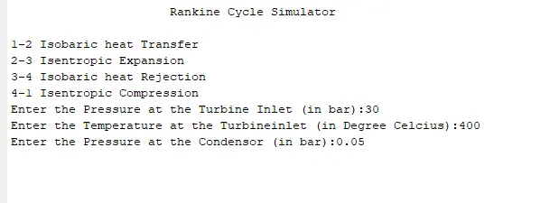
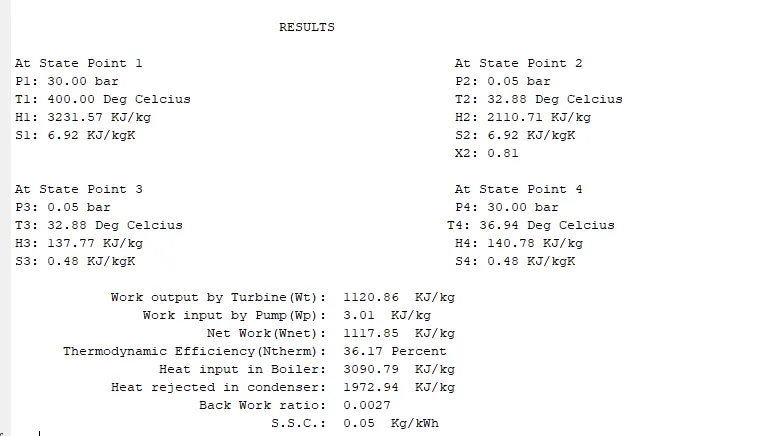
Output Command window:

Output Graphs:

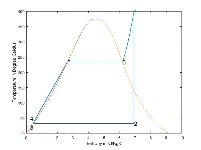
T-s diagram of the Rankine cycle:

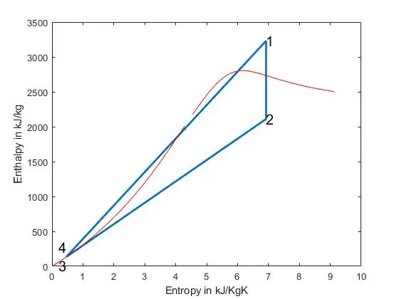
H-s diagram of the Rankine cycle:

Challenges :

If we see both plots we can't see the work done by the pump because it is very small compared to other values it will be only visible if you zoom out the plot between process 5-1.

It was happening because of using the XSteam.m file for finding all the state points and not relying on formulas to calculate state points. If we find values using formulas it will be easily seen on the plot.

So finding this outcome and understanding the reason was a challenge.

Results and Conclusion:

The performance of the Heat Engine was calculated and the following observations were made:

Net Work = 1117.85 kJ/kg

Thermal Efficiency = 36.17%

Back Work Ratio = 0.27%

The T-S and H-S performance curves of the Rankine Cycle were plotted.