Challenge

Optimization of the stalagmite function using the genetic algorithm and to find out the global maxima.

PPranav Upadhyay28 Aug 2020

DETAILED REPORT ON THE GENETIC ALGORITHM CHALLENGE

1. Aim:

To optimize the stalagmite function using the genetic algorithm and to find out the global maxima.

2. Theory:

"A genetic algorithm is a search heuristic that is inspired by Charles Darwin’s theory of natural evolution. This algorithm reflects the process of natural selection where the fittest individuals are selected for reproduction in order to produce offspring of the next generation."

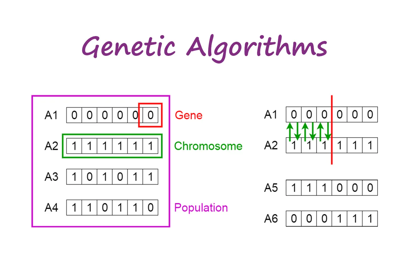
The process of natural selection starts with the selection of fittest individuals from a population. They produce offspring which inherit the characteristics of the parents and will be added to the next generation. If parents have better fitness, their offspring will be better than parents and have a better chance of surviving. This process keeps on iterating and in the end, a generation with the fittest individuals will be found.

This notion can be applied to a search problem. We consider a set of solutions for a problem and select the set of best ones out of them.

Five phases are considered in a genetic algorithm.

Initial population
Fitness function
Selection
Crossover
Mutation

Initial Population

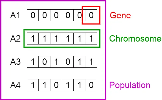
The process begins with a set of individuals which is called a Population. Each individual is a solution to the problem you want to solve.

An individual is characterized by a set of parameters (variables) known as Genes. Genes are joined into a string to form a Chromosome (solution).

In a genetic algorithm, the set of genes of an individual is represented using a string, in terms of an alphabet. Usually, binary values are used (a string of 1s and 0s). We say that we encode the genes in a chromosome.

Fitness Function

The fitness function determines how to fit an individual is (the ability of an individual to compete with other individuals). It gives a fitness score to each individual. The probability that an individual will be selected for reproduction is based on its fitness score.

Selection

The idea of the selection phase is to select the fittest individuals and let them pass their genes to the next generation.

Two pairs of individuals (parents) are selected based on their fitness scores. Individuals with high fitness have more chances to be selected for reproduction.

Crossover

Crossover is the most significant phase in a genetic algorithm. For each pair of parents to be mated, a crossover point is chosen at random from within the genes.

For example, consider the crossover point to be 3 as shown below.

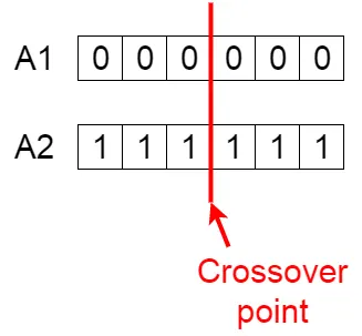
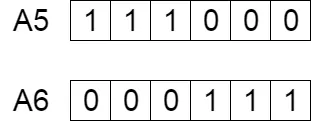
Offspring are created by exchanging the genes of parents among themselves until the crossover point is reached.

The new offspring are added to the population.

Mutation

In certain new offspring formed, some of their genes can be subjected to a mutation with a low random probability. This implies that some of the bits in the bit string can be flipped.

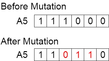
The mutation occurs to maintain diversity within the population and prevent premature convergence.

Termination

The algorithm terminates if the population has converged (does not produce offspring which are significantly different from the previous generation). Then it is said that the genetic algorithm has provided a set of solutions to our problem.

3. Syntax of @ga:

Find a minimum of a function using genetic algorithm

Syntax-

Description-

x = ga(fun,nvars) finds a local unconstrained minimum, x, to the objective function, fun. nvars is the dimension (number of design variables) of fun.
x = ga(fun,nvars,A,b) finds a local minimum x to fun, subject to the linear inequalities A*x ≤ b. ga evaluates the matrix product A*x as if x is transposed (A*x').
x = ga(fun,nvars,A,b,Aeq,beq) finds a local minimum x to fun, subject to the linear equalities Aeq*x = beq and A*x ≤ b. (Set A=[] and b=[] if no linear inequalities exist.) ga evaluates the matrix product Aeq*x as if x is transposed (Aeq*x').
x = ga(fun,nvars,A,b,Aeq,beq,lb,ub) defines a set of lower and upper bounds on the design variables, x, so that a solution is found in the range lb ≤ x ≤ ub. (Set Aeq=[] and beq=[] if no linear equalities exist.)
x = ga(fun,nvars,A,b,Aeq,beq,lb,ub,nonlcon) subjects the minimization to the constraints defined in nonlcon. The function nonlcon accepts x and returns vectors Cand Ceq, representing the nonlinear inequalities and equalities respectively. ga minimizes the fun such that C(x) ≤ 0 and Ceq(x) = 0. (Set lb=[] and ub=[] if no bounds exist.)
x = ga(fun,nvars,A,b,Aeq,beq,lb,ub,nonlcon,options) minimizes with the default optimization parameters replaced by values in options. (Set nonlcon=[] if no nonlinear constraints exist.) Create options using optimoptions.
x = ga(fun,nvars,A,b,[],[],lb,ub,nonlcon,IntCon) or x = ga(fun,nvars,A,b,[],[],lb,ub,nonlcon,IntCon,options) requires that the variables listed in IntCon take integer values.

x = ga(problem) finds the minimum for problem, where problem is a structure.

[x,fval] = ga(___), for any previous input arguments, also returns fval, the value of the fitness function at x.
[x,fval,exitflag,output] = ga(___) also returns exitflag, an integer identifying the reason the algorithm terminated, and output, a structure that contains output from each generation and other information about the performance of the algorithm.
[x,fval,exitflag,output,population,scores] = ga(___) also returns a matrix population, whose rows are the final population, and a vector scores, the scores of the final population.

4. Governing Equations:

`f(x,y)=f_(1,x)*f_(2,x)*f_(1,y)*f_(2,y)`
`f_(1,x) = [sin(5.1pix+0.5)]^6`
`f_(1,y) = [sin(5.1piy+0.5)]^6`
`f_(2,x)=exp[-4ln2(x-0.0667)^2/0.64]`
`f_(2,y)=exp[-4ln2(y-0.0667)^2/0.64]`

5. Stalagmite function:

The codes below are scripted in MATLAB(R2020a)

function [F] = stalagmite(input)
f1x = (sin(5.1*pi*input(1) + 0.5))^6;
f1y = (sin(5.1*pi*input(2) + 0.5))^6;
f2x = exp(-4*log(2)*(((input(1) - 0.0667^2)/(0.64))));
f2y = exp(-4*log(2)*(((input(2) - 0.0667^2)/(0.64))));
F = -(f1x * f1y * f2x * f2y);
end

The above function defines the stalagmite function.
The function accepts an array from the main function and calculates the value using the function definition.
The negative(-) in F, represents the maxima.

6. Optimization:

%% Program
clear all
close all
clc

%% 1) Defining Range
x = linspace(0,0.6,150);                        % range of x
y = linspace(0,0.6,150);                        % range of y

[xx yy] = meshgrid(x,y);                      % creating 2D array of range

iterations = 40;
%% 2) Solving Stalagmite Function
% nested loop is run for the entire range to input each range value one by one.

for i = 1:length(xx)
    for j= 1:length(yy)
        input_vector(1) = xx(i,j);                 % picking values from xx matrix
        input_vector(2) = yy(i,j);                 % picking values from yy matrix
        sol(i,j) = stalagmite(input_vector);       % calling the stalagmite function and proving inputs.
    end
end

%% 2.1) Plotting Stalagmite Function
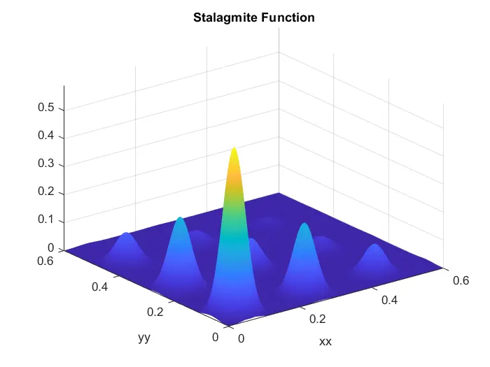
figure(1)
surfc(xx, yy, -sol);                      % plotting the stalagmite functn using the surfc command
shading interp                            % removing the shadings from the plot
xlabel('xx'); ylabel('yy');
title('Stalagmite Function')
%% 3) First Study (Unbound Inputs)
%
% use the for loop to run the itaerations and call the ga function every time
%
tic;                                                % start the timer for first study
for i = 1:iterations;                               % start the loop
    [sol1 fval1(i)] = ga(@stalagmite, 2);           % calling ga function
                                                    % sol1 is the solution
                                                    % and fval1 is the function value
    sol_x1(i) = sol1(1);                               % storing the value of x seperately
    sol_y1(i) = sol1(2);                               % storing the value of y seperately
    clc                                             % clearing the command window after each iteration.
end
study1_time = toc;                                  % stopping the timer

%% 3.1) Plotting First Study
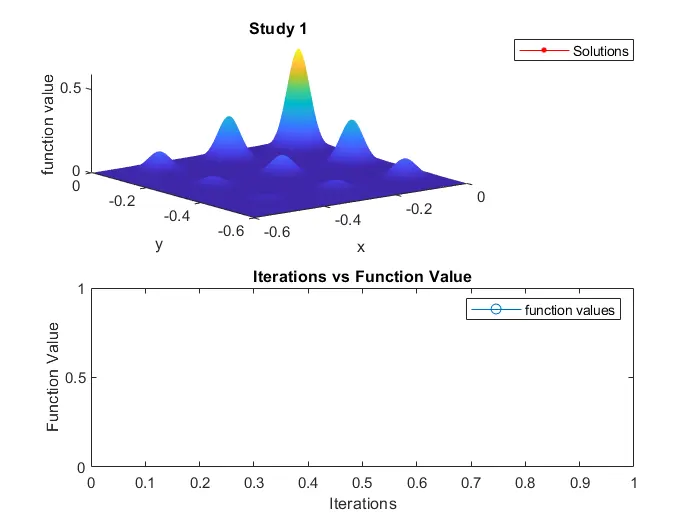
figure(2)
subplot(2,1,1);                                                  % creating first half of the figure

plot3(-sol_x1, -sol_y1, -fval1,'- .','markersize',10,'color','r')     % plotting the solution of first study
xlabel('x'); ylabel('y'); zlabel('function value');              % labelling the axes
title('Study 1');                                                % title of the plot
hold on                                                          % holding the next plots


surfc(-xx,-yy,-sol);                                                % plotting the stalagmite function
shading interp;                                                  % removing the shading from the plot
legend('Solutions')

subplot(2,1,2);                                                  % creating second half of the figure
plot(fval1,'-o');                                                % plotting the function values
title('Iterations vs Function Value');                           % title of the plot
xlabel('Iterations'); ylabel('Function Value');                  % labelling the axes
legend('function values')
hold off
%% 4) Second Study (Bounded Inputs)
%
% use the for loop to run the iterations and also provide the lower and upper bounds
%
tic;                                                                          
for i = 1:iterations                                                    % starting the timer
    [sol2 fval2(i)] = ga(@stalagmite, 2,[],[],[],[],[0;0],[1;1]);       % calling the ga function
    sol_x2(i) = sol2(1);
    sol_y2(i) = sol2(2);                                                % storing x and y values seperately
    clc                                                                 % clearing command window on each iteration
end
study2_time = toc;                                                      % stooping the study timer

%% 4.1) Plotting Second Study
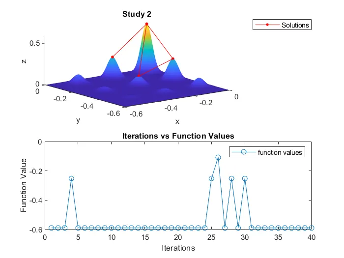
figure(3)
subplot(2,1,1);                                                         % generating the upper half of the figure

plot3(-sol_x2,-sol_y2,-fval2,'- .','markersize',10,'color','r');             % plotting the solution of the function
title('Study 2');                                                       % title of plot
xlabel('x'); ylabel('y'); zlabel('z');                                  % labelling the axes
hold on

surfc(-xx, -yy, -sol);                                                     % plotting the stalgmite function
shading interp;
legend('Solutions')                                                     % inseting the required legends

subplot(2,1,2);                                                         % generating the lower half of the plot
plot(fval2,'-o');                                                       % plotting the function values
xlabel('Iterations'); ylabel('Function Value');                         % labelling the axes
title('Iterations vs Function Values');                                 % title of the plot
legend('function values')                                               % inserting required legends
hold off
%% 5) Third Study (Bounded Inputs with Population Size')
tic;                                                                           % starting the study timer

options = optimoptions('ga');                                                  % initializing options
options = optimoptions('ga','PopulationSize',500);                             % proving options parameters using optimoptions function

% now ga will maximize the default optimization parameters replaced by values in options
for i = 1:iterations                                                            % starting the loop
    [sol3 fval3(i)] = ga(@stalagmite, 2,[],[],[],[],[0;0],[1;1],[],options);    % solving the stalagmite function
    sol_x3(i) = sol3(1);                                                        % seperating x and y values
    sol_y3(i) = sol3(2); 
    clc                                                                         % clearing command window on each iteration
end
study3_time = toc;                                                              % stopping the timer

%% 5.1) Plotting the third Study
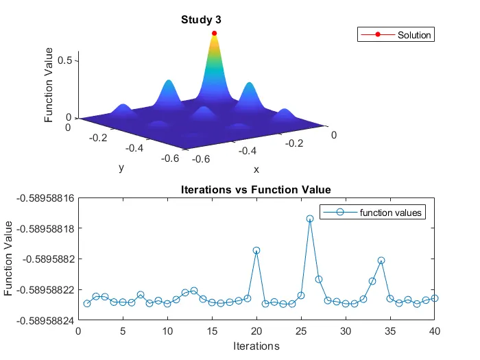
figure(4)
subplot(2,1,1);                                                        % generating the upper half of the plot

plot3(-sol_x3, -sol_y3, -fval3,'- .','markersize',15,'color','r');          % plotting the solution
xlabel('x'); ylabel('y'); zlabel('Function Value');                    % labelling the axes
title('Study 3');                                                      % title of the plot
hold on

surfc(-xx,-yy,-sol);                                                      % plotting th stalagmite function
shading interp;                         
legend('Solution')                                                     % inserting required legends

subplot(2,1,2);                                                        % generating lower half of the plot
plot(fval3,'-o');                                                      % plotting the function values
xlabel('Iterations'); ylabel('Function Value');                        % labelling the axes
title('Iterations vs Function Value');                                 % title of the plot
legend('function values')                                              % inserting legendd
hold off

%% Displaying Soluton Outputs
disp('------------------------------Maximized Stalagmite Function------------------------------')

disp('Solution Values :')                    % displaying value of solution obtained after third study 
disp(' ')
disp(sol_x3)                               % values of x (input_vector(1))
disp(' ')
disp(sol_y3)                               % values of y (input_vector(2))
disp('Function Values :') 
disp(' ')
disp(fval3)                                % displaying function values
disp(' ')
disp('------------------------------Time taken for each study------------------------------')
fprintf('nTime taken for first study = %f secondsnn',study1_time)     % displaying time taken for all three studies
fprintf('Time taken for second study = %f secondsnn',study2_time)
fprintf('Time taken for third study = %f secondsnn',study3_time)

7. Results:

8. Conclusion:

The required optimization is done and results are as shown above.

Time taken for first study = 0.731916 seconds
Time taken for second study = 4.056662 seconds
Time taken for third study = 24.663283 seconds

Optimization of the stalagmite function using the genetic algorithm and to find out the global maxima.

Initial Population

Fitness Function

Selection

Crossover

Mutation

Termination

Ship work like this
in your own course.

Talk to a career counsellor

Initial Population

Fitness Function

Selection

Crossover

Mutation

Termination

Ship work like thisin your own course.

Talk to a career counsellor

Ship work like this
in your own course.