Solving second order Ordinary Differential Equation to simulate the motion of a Simple Pendulum using MATLAB.

DETAILED REPORT ON THE SECOND ORDER ODE

1. AIM:

• The aim of this challenge is to solve a second-order ordinary differential equation and simulate the motion of a pendulum obtained as a result of the solution obtained.

2. OBJECTIVES:

• To solve a second order ODE.
• To understand how an ODE is solved using MATLAB tools.
• To program a function in MATLAB able to output a position of the pendulum in radians with respect to time.
• To prepare a simulation showing the position of the pendulum based on certain entered criteria such as damping coefficient, gravity, length of the pendulum, and mass of the pendulum.

3. GOVERNING EQUATION:

1. `(d^2theta)/(d^2t) + b/m ((d theta) /dt) + g/L sin theta = 0`, this ODE represents the motion of a simple using with damping.
2. where b is the damping coefficient.
3. g is gravity.
4. L is the length of the pendulum.
5. m is the mass of the bob.

4. EXPLANATION:

• The following code is written in MATLAB (R2020a).
• Below is the MATLAB script for the ODE solver and code for simulating the motion of the pendulum.

% Program to solve the ode and simulate the motion of a pendulum.
close all
clear all
clc

% Declaring constants and initialising the values.
b=0.005;
g=9.81;
l=1;
m=1;

% Defining the parameters
theta_0 = [0;5];
t_span = linspace(0,10,500);
% Function calling statement.
[t,results] = ode45(@(t,theta) ode_func(t,theta,b,g,l,m),t_span,theta_0);

% Plotting the curve
figure(1)
plot(t,results(:,1))
hold on
plot(t,results(:,2))
ylabel('Plot')
xlabel('Time')

%Simulation of the pendulum
ct =1;
for i = 1:length(results(:,1))
    x0=0;
    y0=0;
    x1 = l* sin(results(i,1));
    y1 = -l* cos(results(i,1));
    figure(2)
    plot([-1 1],[0 0],'linewidth',4,'color','k')
    axis([-2 2 -2 2]);
    hold on
    line([x0 x1],[y0 y1],'linewidth',2,'color','b')
    hold on
    plot(x1,y1,'.','markersize',30,'color','r')
    grid on
    hold off
    M(ct) = getframe(gcf);
    ct = ct+1;
end

% Creating animation
movie(M)
videofile = VideoWriter('Pendulum_Movement.avi','Uncompressed AVI');
open(videofile)
writeVideo(videofile,M)
close(videofile)

In the above code:

• first of all, the constants are declared and initialized.
• Now initial conditions are defined.
• theta_0 is a two-column vector, it stores, position in the first column and the velocity is stored in the second column.
• t_span is the total time period.
• To solve the ODE, the ode45 function is used.
• The function definition is shown below.

function [dtheta_dt] = ode_func(t,theta,b,g,l,m)
theta1 = theta(1);
theta2 = theta(2);
dtheta1_dt = theta2;
dtheta2_dt = -(b/m)*theta2 - (g/l)*sin(theta1);
dtheta_dt = [dtheta1_dt;dtheta2_dt];
end

• The above function declaration is called in the main Matlab script.
• The function returns two values, t and results.
• t store the time and the result is a two-column matrix.
• First-column store theta and the second-column store velocity.
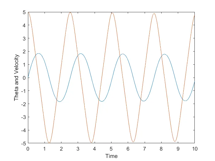
• Now, position and velocity are plotted against time using plot() function.

5. SIMULATING THE MOTION OF THE PENDULUM:

%Simulation of the pendulum
ct =1;
for i = 1:length(results(:,1))
    x0=0;                                            % the fixed point of the pendulum
    y0=0;
    x1 = l* sin(results(i,1));                       % the point representing the position of bob
    y1 = -l* cos(results(i,1));
    figure(2)
    plot([-1 1],[0 0],'linewidth',4,'color','k')
    axis([-2 2 -2 2]);
    hold on
    line([x0 x1],[y0 y1],'linewidth',2,'color','b')
    hold on
    plot(x1,y1,'.','markersize',30,'color','r')
    grid on
    hold off
    M(ct) = getframe(gcf);
    ct = ct+1;
end

• The above code bloc successfully simulates the motion of pendulum in MATLAB.
• ct is a counter variable and is increased by 1 for every successive iteration. It is used to store a particular frame in the M array with the help of getframe() function which uses the current figure and store it in M.
• for loop, I have the length function. It returns a positive integer value of the total size of an array.
• In this case, I have iterated for the (total number of values stored in result array) times.
• for every successive value of results, x1 and y1 are calculated as written in the code.
• plot([-1 1],[0 0],'linewidth',4,'color','k'), this line is used to draw a surface from the pendulum is attached(a rigid support).
• axis function is used to define the axes.
• marker is used to represent the bob with increased size.

6. CONCLUSION:

The following outputs are obtained as result of the above codes.

• A plot for Position and velocity vs time is plotted successfully.
• A simulation for the motion of a pendulum is done successfully.