Rankine cycle Simulator

DETAILED REPORT ON THE RANKINE CYCLE SIMULATOR

1. AIM:

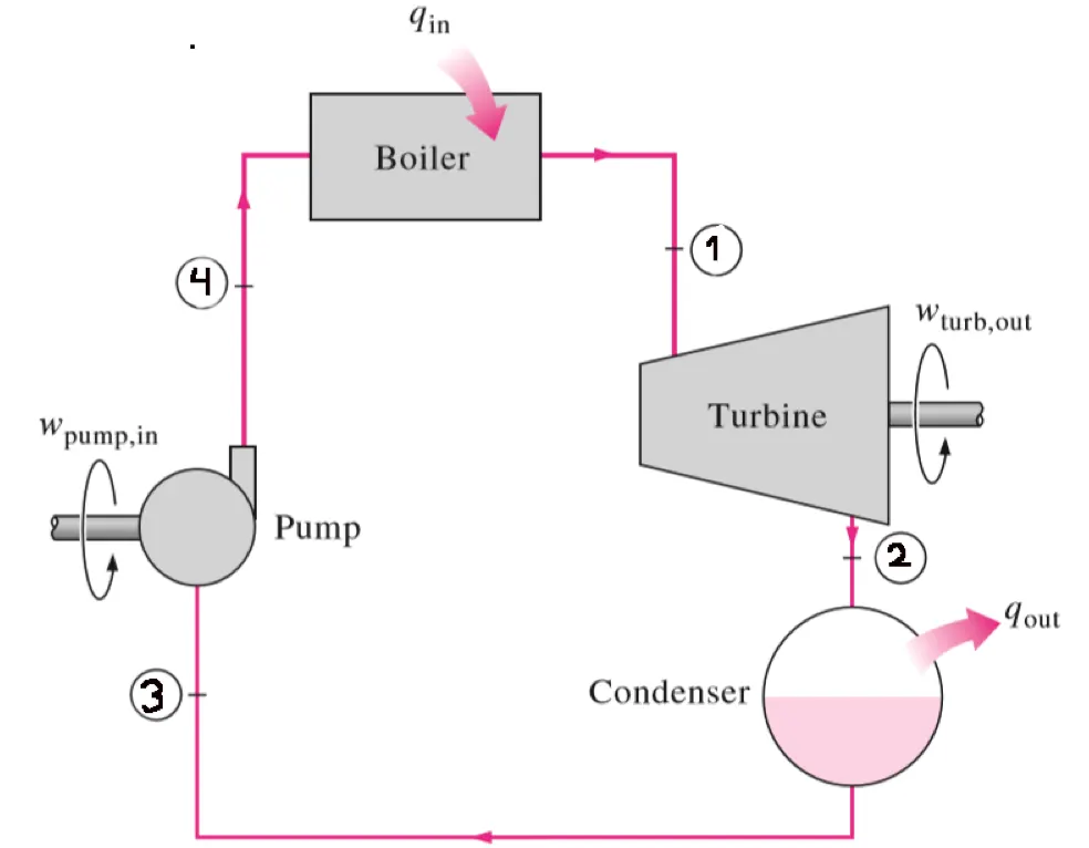
The objective here is to simulate an Ideal Rankine Cycle

2. Theory:

Many of the impracticalities associated with the Carnot cycle can be eliminated by superheating the steam in the boiler and condensing it completely in the condenser. The cycle that results is the Rankine cycle, which is the ideal cycle for vapor power plants. The ideal Rankine cycle does not involve any internal irreversibilities and consists of the following four processes:

1-2: Isentropic expansion in the turbine
2-3: Isobaric heat rejection in the condenser
3-4: Isentropic compression in the pump
4-1: Isobaric heat addition in the boiler

3. INPUTS:

Xsteam Library

Pressure at the turbine inlet (in bar): 30
Temperature at the Turbine inlet (in Degree Celsius): 400
Pressure at the Condenser (in bar): 0.05

4. CODE:

• The following code has been written in MATLAB(R 2020a).

% RANKINE CYCLE SIMULATOR

clear all 
close all 
clc

% Printing name of the cycle and processes

fprintf('IDEAL RANKINE CYCLE SIMULATOR n n n')
fprintf('Line 1-2 : Isentropic expansion in turbine n')
fprintf('Line 2-3 : Isobaric heat rejection in the condenser n')
fprintf('line 3-4 : Isentropic compression in the pump n') 
fprintf('Line 4-1: Isobaric heat addition in boiler n n')

%Inputs

P1 = input('Pressure at the turbine inlet (in bar): '); 
T1 =input('Temperature at the Turbine inlet (in Degree Celsius): ');
P2 = input('Pressure at the Condenser (in bar): ');
disp(' ')
disp('Outputs')

% At state point 1

disp('At state point 1:')
fprintf('P1 : %g Bar n', P1)
fprintf('T1 : %g Deg Celcius n', T1)
H1 = XSteam('h_pt', P1, T1);
fprintf('H1: %g kJ/kg n', H1)
S1 = XSteam('s_pt', P1, T1);
fprintf('S1 : %g kJ/kgk n n', S1)

% At state point 2

disp('At state point 2: ')
fprintf('P2 : %g Bar n', P2)
S2 = S1;
fprintf('S2 : %g kJ/kgk n', S2)
Sg = XSteam('sV_p', P2);
Sf = XSteam('SL_p', P2);
Sfg = Sg - Sf;
X2 = (S2 - Sf) / (Sfg);
fprintf('X2 : %g n', X2)
Hf = XSteam('hL_p', P2);
Hg = XSteam('hV_p', P2);
Hfg = Hg - Hf;
H2 = Hf + X2 * Hfg;
fprintf('H2 is : %g kJ/kg n', H2)
T2 = XSteam('Tsat_p', P2); 
fprintf('T2 : %g Deg Celcius n n', T2)

% At state point 3

disp('At state point 3: ')
P3 = P2;
fprintf('P3: %g Bar n', P3) 
V3 = XSteam('vL_p', P3);
T3 = T2;
fprintf('T3 : %g Deg Celcius n', T3)
H3 = XSteam('hL_p', P3);
fprintf('H3: %g kJ/kg n', H3)
S3 = XSteam('sL_p', P3); 
fprintf('S3: %g kJ/kgK n n', S3)

% At state point 4

disp('At state point 4: ')
P4 = P1;
fprintf('P4 : %g Bar n', P4)
S4 = S3;
fprintf('S4 : %g kJ/kgK n', S4)
W_pump = V3 * (P4 - P3) * 100;
H4 = W_pump + H3;
fprintf('H4 : %g kJ/kg n', H4)
T4 = XSteam('T_ps', P4, S4);
fprintf('T4 : %g Deg Celcius n n', T4)

% At Calculating the efficiency of cycle and specific steam consumption

W_Turbine = H1 - H2;
fprintf('W_Turbine: %g kJ/kg n', W_Turbine)
fprintf('W_pump : %g kJ/kg n', W_pump)
W_Net = W_Turbine - W_pump;
fprintf('W_net : %g kJ/kg n', W_Net)
Q_in = H1 - H4;
Efficiency_thermo = W_Net / Q_in * 1e2;
fprintf('Efficiency_thermo: %g', Efficiency_thermo);
disp('%')
S_S_C = 3600 / W_Turbine;
fprintf('S_S_C : %g kg/KWh n n', S_S_C)

% Plotting liquid line and vapour

temp = linspace(1, 373, 500);
for i = 1 : length(temp)
H_L(i) = XSteam('hL_T', temp(i));
H_V(i) = XSteam('hV_T', temp(i));
S_L(i) = XSteam('sL_T', temp(i));
S_V(i) = XSteam('sV_T', temp(i));
end

%Points between state point 4 to state point 1

S5 = XSteam('sL_p', P1);
S6 = XSteam('sV_p', P1);
T5 = XSteam('Tsat_p', P1);
T6 = XSteam('Tsat_p', P1);

% Plotting T - S and H - S Diagrams

figure(1)
hold on
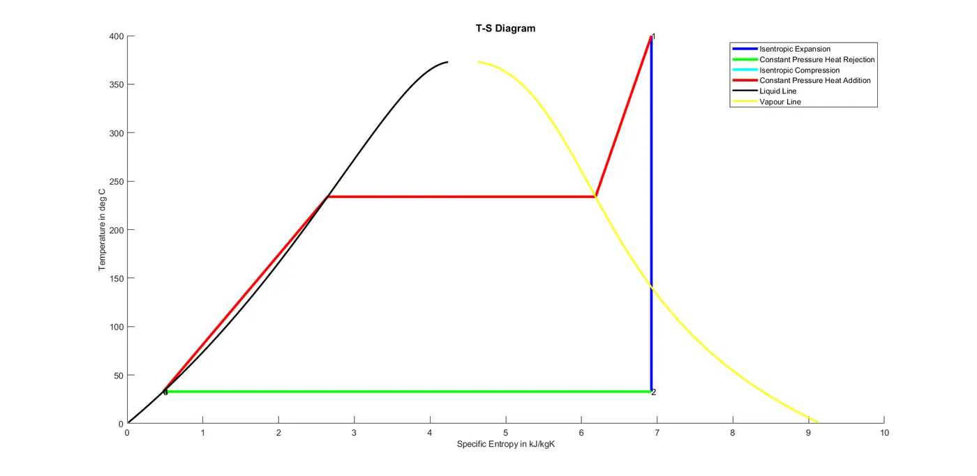
plot ([S1 S2],[T1 T2], 'b', 'linewidth', 3) 
plot([S2 S3],[T2 T3], 'g', 'linewidth',3)
plot([S3 S4],[T3 T4], 'c', 'linewidth',3)
plot([S4 S5 S6 S1], [T4 T5 T6 T1], 'r', 'linewidth',3) 
plot (S_L, temp, 'k', 'linewidth',2)
plot (S_V, temp, 'y', 'linewidth',2)
%Indicating state points with numbers
text(S1, T1, '1');
text(S2, T2,'2');
text(S3,T3,'3'); 
text(S4, T4,'4');
legend('Isentropic Expansion',...
'Constant Pressure Heat Rejection',...
'Isentropic Compression',...
'Constant Pressure Heat Addition',...
'Liquid Line', 'Vapour Line');
title('T-S Diagram', 'FontSize', 12) 
xlabel('Specific Entropy in kJ/kgK', 'FontSize',10)
ylabel('Temperature in deg C', 'FontSize',10)

figure(2)
hold on
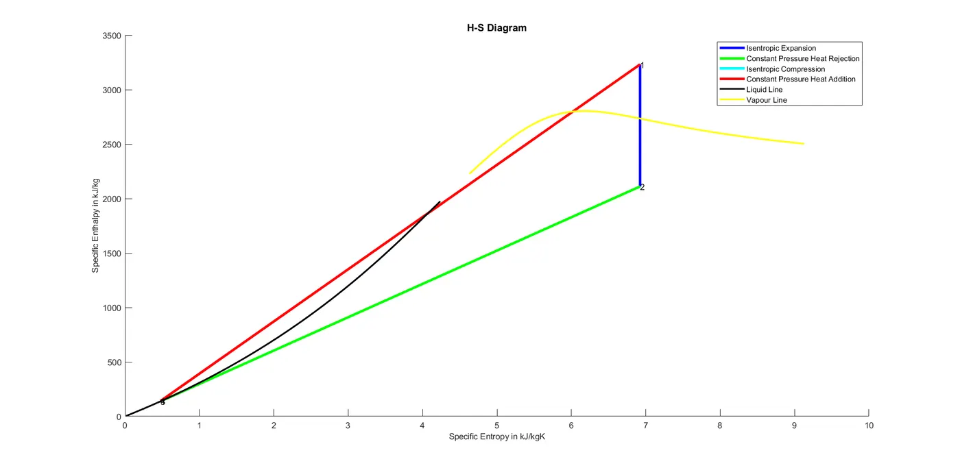
plot ([S1 S2], [H1 H2], 'b', 'linewidth',3);
plot ([S2 S3], [H2 H3],'g', 'linewidth',3);
plot ([S3 S4], [H3 H4], 'c', 'linewidth', 3); 
plot ([S4 S1], [H4 H1], 'r','linewidth', 3);
plot (S_L, H_L,'k','linewidth',2) 
plot (S_V, H_V, 'y', 'linewidth', 2)
%Indicating state points with numbers 
text(S1, H1, '1');
text(S2, H2, '2');
text(S3, H3,'3'); 
text(S4, H4, '4');
legend('Isentropic Expansion',...
'Constant Pressure Heat Rejection',...
'Isentropic Compression',...
'Constant Pressure Heat Addition', ...
'Liquid Line', 'Vapour Line');
title('H-S Diagram', 'FontSize', 12)
ylabel('Specific Enthalpy in kJ/kg','FontSize',10) 
xlabel('Specific Entropy in kJ/kgK','FontSize',10)

5. EXPLANATIONS:

1-2: Isentropic expansion in the turbine

In this process, the superheated steam enters the turbine and expands isentropically. As a result of which a certain amount of work is done by the turbine(`W_t`). The shaft of the turbine is connected to the generator. hence, the mechanical here is converted into useful energy.

`W_t = m* (h_1-h_2)*K`

2-3: Isobaric heat rejection in the condenser

In this process, expanded vapour is then passed through the condenser and some amount of heat is rejected`(Q_r)`. Then vapour gets converted into liquid and hence is pumped up again into the cycle.

`Q_r = m*(h_2- h_3)*K`

3-4: Isentropic compression in the pump

In this process, water into the pump in saturated form and here it is compressed isentropically until it reaches the boiler temperature. Some work(`W_p`) is done by the pump too.

`W_p = m*(h_3-h_4)*K`

4-1: Isobaric heat addition in the boiler

In this process, water enters into the boiler, and leaves into its superheated phase.

`Q_a = m*(h_1-h_4)*K`

6. OUTPUTS:

W_Turbine: 1120.86 kJ/kg
W_pump: 3.01094 kJ/kg
W_net: 1117.85 kJ/kg
Efficiency_thermo: 36.1671%
S_S_C: 3.21181 kg/KWh

7. REFERENCES:

• Thermodynamics: An Engineering Approach, 5th edition, Yunus A. Cengel and Micheal A. Boles

• https://skill-lync.com/projects/rankine-cycle-simulator-101

• https://en.wikipedia.org/wiki/Rankine_cycle#:~:text=The%20Rankine%20cycle%20is%20an,the%20four%20components%20are%20neglected.