Higher Order Polynomial vs Split wise Curve Fitting Using MATLAB

CURVE FITTING

AIM: Write code to fit a linear and cubic polynomial for the Cp data.

OBJECTIVES:

• Plot the linear and cubic fit curves along with the raw data points. Title and axes labels are a must, legends could be shown if necessary.
• Write a code to show split wise method.
• Explain the parameters used to measure the fitness characteristics for both the curves.

THEORY:

• Curve fitting is the process of constructing a curve, or Mathematical function, that has the best fit to a series of data points, possibly subject to constraints.
• Curve fitting can involve either interpolation, where an exact fit to the data is required, or smoothing, in which a "smooth" function is constructed that approximately fits the data. A related topic is regression analysis, which focuses more on questions of statistical inference such as how much uncertainty is present in a curve that is fit to data observed with random errors.
• Fitted curves can be used as an aid for data visualization, to infer values of a function where no data are available, and to summarize the relationships among two or more variables

Linear curve fit:

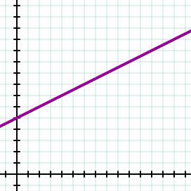
• A combination of constant and direct. A fixed amount is added (or subtracted) at regular intervals.

General form, y = ax + b

A suitable conclusion statement from such a relationship would be that…

• y is linear with x.
• y varies linearly with x.
• y is a linear function of x.

Appearance: any straight line, regardless of slope or y-intercept

Cubic curve fit:

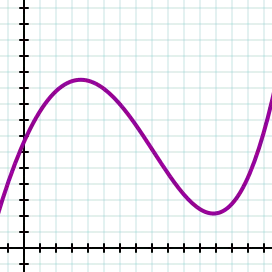
• A combination of a constant, direct, square & cube.

General form, `y = a + bx + cx^2 + dx^3`

A suitable conclusion statement from such a relationship would be that…

• y can be approximated by a third order polynomial of x.
• y is a cubic function of x.

Appearance: any non-periodic function without asymptotes.

Parameters used to measure the fitness characteristics of curve fit:

• After fitting data with one or more models, you should evaluate the goodness of fit. A visual examination of the fitted curve displayed in the Curve Fitting Tool should be your first step
• You can group these measures into two types: graphical and numerical. The residuals and prediction bounds are graphical measures, while the goodness of fit statistics and confidence bounds are numerical measures.
• Graphical measures are more beneficial than numerical measures because they allow you to view the entire data set at once, and they can easily display a wide range of relationships between the model and the data.
• The numerical measures are more narrowly focused on a particular aspect of the data and often try to compress that information into a single number.
• In practice, depending on your data and analysis requirements, you might need to use both types to determine the best fit

Goodness of Fit Statistics

• After using graphical methods to evaluate the goodness of fit, you should examine the goodness of fit statistics. The Curve Fitting Toolbox supports this goodness of fit statistics for parametric models:

• The sum of squares due to error (SSE)
• R-square
• Adjusted R-square
• Root mean squared error (RMSE)

• Sum of Squares Due to Error (SSE): This statistic measures the total deviation of the response values from the fit to the response values. It is also called the summed square of residuals and is usually labelled as SSE

`SSE = sum_(i=1)^n(Y(i)-f(x(i)))^2`

A value closer to 0 indicates a better fit.

• R-square: This statistic measures how successful the fit is in explaining the variation of the data. Put another way, R-square is the square of the correlation between the response values and the predicted response values. It is also called the square of the multiple correlation coefficient and the coefficient of multiple determination.

R-square is defined as the ratio of the sum of squares of the regression (SSR) and the total sum of squares (SST). SSR is defined as,

`R^2 = (SSR)/(SST)`

R-square can take on any value between 0 and 1, with a value closer to 1 indicating a better fit.

were,

SSR: which is basically the square of the difference between the value of the fitting function at a given point and the arithmetic mean of the data set.

`SSR = sum_(i=1)^n(f(x(i))-Mean)^2`

SST : SST is also called the sum of squares about the mean.

`SST=SSR+SSE`

• Adjusted R-square: This statistic uses the R-square statistic defined above, and adjusts it based on the residual degrees of freedom. The residual degrees of freedom are defined as the number of response values n minus the number of fitted coefficients m estimated from the response values

The adjusted R-square statistic is generally the best indicator of the fit quality when you add additional coefficients to your model.

The adjusted R-square statistic can take on any value less than or equal to 1, with a value closer to 1 indicating a better fit

• Root Mean Squared Error (RMSE): This statistic is also known as the fit standard error and the standard error of the regression

It is an estimate of the standard deviation of the random component in the data, and is defined as,

`RMSE = sqrt((sum_(i=1)^n(Y(i)-f(x(i)))^2)/n) = sqrt((SSE)/n)`

where, n is the total number of datapoints available

A RMSE value closer to 0 indicates a better fit.

Using these four quantities MATLAB effectively deduces the goodness of fit, typically is R-square is greater than 0.95 the fit is assumed to be good.

GOVERNING EQUATIONS:

Parameters used to measure the fitness characteristics of curve fit

Fitting function, `y = f(x)`

• Error

`"Error" = abs(Y(i) - f(x(i))`

`Y(i)` = value of the fitting function

`f(x(i))` = original data set

• SSE

`SSE = sum_(i=1)^n(Y(i)-f(x(i)))^2`

`Y(i)` = value of the fitting function

`f(x(i))` = original data set

• SSR

`SSR = sum_(i=1)^n(f(x(i))-Mean)^2`

`f(x(i))`= value of the fitting function

mean = arithmetic means of the data set

• SST

`SST=SSR+SSE`

• R-square

`R^2 = (SSR)/(SST)`

• RMSE

`RMSE = sqrt((SSE)/n)`

n = number of datapoints

PROCEDURE:

• In concern to our objectives, we need to curve fit the data in 3 methods. Linear curve fit, cubic curve fit and curve fit using split wise method.
• so, we are going to code 2 programs, one for curve fit the data using linear curve fit and cubic curve fit and measures its goodness.
• Another program for curve fit the data using split wise method and analysing goodness of the curve.
• For both programs, we need to load our data file in to MATLAB. after that we need to separate temperature and cps in to two different arrays.
• Find coefficients for our polynomial function and create polynomial values, which is our predicted cp values.
• plot both data point and curve fit.
• for analysing goodness of our curve fit, we could use curve fitting toolbox available on MATLAB.
• But in our program, we are going to calculate the parameters using governed equations
• we need to print the calculated goodness parameters as results and need to valuate goodness of the curve.

Input file for our program is Temperature vs cp data file (click here)

PROGRAM:

1.Linear and cubic curve fit

%PROGRAM FOR LINEAR AND CUBIC CURVE FITTING 
clear all 
close all
clc

%Preparing the data
cp_file = load('data');
%Temperature [Kelvin]
temperature = cp_file(:,1);
%Specific heat [KJ/Kmol-K]
cp = cp_file(:,2);

%Linear curve fit
%finding coefficents for linear polynamial function
%f(x)=Ax+B; %A,B = Coefficients
coeffs_l = polyfit(temperature,cp,1);
%calculating cp using linear polynamial function
cp_predicted1 = polyval(coeffs_l,temperature);

%Cubic curve fit
%finding coefficents for cubic polynamial function
%f(x)=A(x^3)+B(x^2)+C(x)+D; %A,B,C,D = Coefficients
coeffs_c = polyfit(temperature,cp,3);
%calculating cp using cubic polynamial function
cp_predicted2 = polyval(coeffs_c,temperature);

%Plotting linear fit curves along with the raw data points
figure(1)
plot(temperature,cp,'linewidth',2);
hold on
plot(temperature,cp_predicted1,'r','LineWidth',2)
xlabel('Temperature [K]')
ylabel('Specific Heat [KJ/Kmol-K]')
legend('original data','curve fit')
title('Linear curve fit')
grid on

%Plotting cubic fit curves along with the raw data points
figure(2)
plot(temperature,cp,'linewidth',2);
hold on
plot(temperature,cp_predicted2,'m','LineWidth',2)
xlabel('Temperature [K]')
ylabel('Specific Heat [KJ/Kmol-K]')
legend('original data','curve fit')
title('Cubic curve fit')
grid on

%Calculating fitness characteristics
n = length(cp);
a = sum(cp);
mean = a/n;
%for linear curve fit
error1 = cp - cp_predicted1;
%SSE
sse1 = error1.^2;
SSE1 = sum(sse1);
%SSR
ssr1 = (cp_predicted1 - mean).^2;
SSR1 = sum(ssr1);
%SST
SST1 = SSR1 + SSE1;
%R-Square
R_sq1 = (SSR1/SST1);
%RMSE
RMSE1 = (SSE1/n)^0.5;
%Finding curve is good fit or not
Goodness_Linear = table(SSE1,SSR1,SST1,R_sq1,RMSE1,'VariableNames',{'SSE','SSR','SST','R^2','RMSE'})  
fprintf('R^2 = %f n',R_sq1)
if (R_sq1 > 0.95)
    disp('Linear curve fit is GOOD FIT')
else
    disp('Linear curve fit is not a GOOD FIT')
end

%for Cubic curve fit
error2 = cp - cp_predicted2;
%SSE
sse2 = error2.^2;
SSE2 = sum(sse2);
%SSR
ssr2 = (cp_predicted2 - mean).^2;
SSR2 = sum(ssr2);
%SST
SST2 = SSR2 + SSE2;
%R-Square
R_sq2 = (SSR2/SST2);
%RMSE
RMSE2 = (SSE2/n)^0.5;
%Finding curve is good fit or not
Goodness_Cubic = table(SSE2,SSR2,SST2,R_sq2,RMSE2,'VariableNames',{'SSE','SSR','SST','R^2','RMSE'})
fprintf('R^2 = %f n',R_sq2)
if (R_sq2 > 0.95)
    disp('Cubic curve fit is GOOD FIT')
else
    disp('Cubic curve fit is not a GOOD FIT')
end

1.1 code Explanation:

• Start this code by clear all, close all, clc we use these commands to clear the workspace off any previously used variables.
• Load the given input data file to MATLAB using load command.
• prepare the data for curve fit by separating the values of temperatures and cps from the data set.
• For linear curve fit, the coefficients of the polynomial relation f(x) = Ax+B .i.e. A, B are calculated by using polyfit command and assigned it in to a variable.
• after finding the coefficients, calculate our new predicted values for cps using polyval command, here we need to give the variable having coefficients and our temperature data
• now we have temperature points as well as predicted cp values for the linear polynomial function.
• plot the given data and predicted data on same figure window for comparison
• same procedures are repeated for calculating curve points for cubic curve fit, cubic curve fit is plotted along with original data points.
• polyfit(x,y,n) is the deciding command which n refers to nth order polynomial function, by varying the n we can curve fit using different polynomial functions
• For Evaluating goodness of our curves, fitness characteristics are calculated using governed equations.
• And for display the calculated values in a table on command window, table command is used
• As the value of R_square is greater than 0.95, our curve fit will be a good fit.
• so the condition is applied using if else command and the result is displayed on command window.

*No major errors were thrown in command window while coding

RESULTS:

Plots:

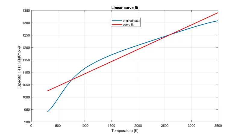
1. Linear curve fit

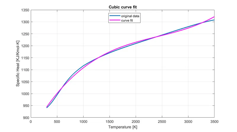
2. Cubic curve fit

Command window:

Curve fitting Toolbox:

PROGRAM:

2. Curve fit using Split wise Method

%PROGRAM TO CURVE FIT USING SPLITWISE METHOD
clear all
close all
clc 

%Preparing the data
cp_file = load('data');
temperature = cp_file(:,1);
cp = cp_file(:,2);

%Splitting Temperatures [Kelvin]
temperature1 = cp_file(1:400,1);
temperature2 = cp_file(401:800,1);
temperature3 = cp_file(801:1600,1);
temperature4 = cp_file(1601:2400,1);
temperature5 = cp_file(2401:3200,1);
%Splitting Specific heats [KJ/Kmol-K]
cp1 = cp_file(1:400,2);
cp2 = cp_file(401:800,2);
cp3 = cp_file(801:1600,2);
cp4 = cp_file(1601:2400,2);
cp5 = cp_file(2401:3200,2);

%curvefitting
%range1
coeffs1 = polyfit(temperature1,cp1,3);
cp_predicted1 = polyval(coeffs1,temperature1);
%range2
coeffs2 = polyfit(temperature2,cp2,2);
cp_predicted2= polyval(coeffs2,temperature2);
%range3
coeffs3 = polyfit(temperature3,cp3,3);
cp_predicted3 = polyval(coeffs3,temperature3);
%range4
coeffs4 = polyfit(temperature4,cp4,2);
cp_predicted4 = polyval(coeffs4,temperature4);
%range5
coeffs5 = polyfit(temperature5,cp5,2);
cp_predicted5 = polyval(coeffs5,temperature5);
%Cp predicted
cp_predicted = [cp_predicted1;cp_predicted2;cp_predicted3;cp_predicted4;cp_predicted5];

%plotting curvefit
plot(temperature,cp,'*','linewidth',2);
hold on
plot(temperature,cp_predicted,'r','LineWidth',2)
xlabel('Temperature [K]')
ylabel('Specific Heat [KJ/Kmol-K]')
legend('original data','curve fit')
title('curve fit - splitwise method')
grid on

%Calculating fitness characteristics
%for splitwise curve fit
n = length(cp);
a = sum(cp);
mean = a/n;
error = cp - cp_predicted;
error_avg = sum(error)/n;
%SSE
sse = error.^2;
SSE = sum(sse);
%SSR
ssr = (cp_predicted - mean).^2;
SSR = sum(ssr);
%SST
SST = SSR + SSE;
%RMSE
RMSE = (SSE/n)^0.5;
%R-Square
R_sq = (SSR/SST);
%Finding curve is good fit or not
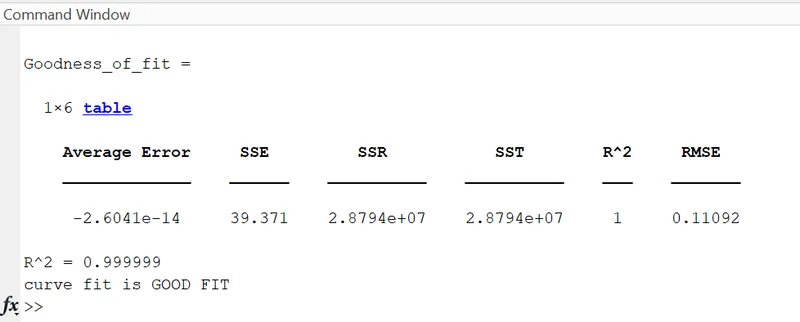
Goodness_of_fit = table(error_avg,SSE,SSR,SST,R_sq,RMSE,'VariableNames',{'Average Error','SSE','SSR','SST','R^2','RMSE'})
fprintf('R^2 = %f n',R_sq)
if (R_sq > 0.95)
    disp('curve fit is GOOD FIT')
else
    disp('curve fit is not a GOOD FIT')
end

2.1 Code explanation

• Start this code by clear all, close all, clc we use these commands to clear the workspace off any previously used variables.
• Load the given input data file to MATLAB using load command.
• prepare the data for curve fit by separating the values of temperatures and cps from the data set.
• Here, we are splitting the data of temperature and cps from the given data file in to 5 ranges of temperatures and cps
• For each range of temperatures and cps, the coefficients are calculated by using polyfit command and assigned it in to a variable.
• after finding the coefficients for each range, calculate new predicted values for cps for all ranges.
• The order of polynomial function for each case can be adjusted, for which the error is to be minimum
• The cps calculated by using polynomial function on each range are aligned to a single array, which is our new predicted data of cps for all temperature range.
• plot the predicted data with original data for comparison
• curve is evaluating using governing equations and results are printed
• for display the calculated values in a table on command window, table command is used
• As the value of R_square is greater than 0.95, our curve fit will be a good fit.
• so the condition is applied using if else command and the result is displayed on command window.

*No major errors were thrown in command window while coding

RESULTS:

Plots:

Command window:

CONCLUSION:

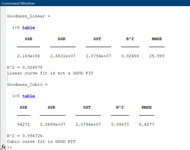
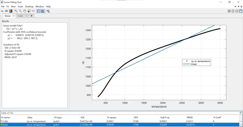
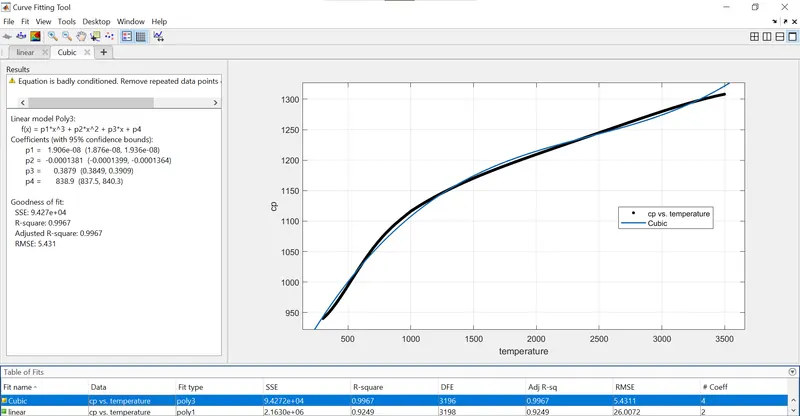
• The value of R-square for Linear fit is found to be 0.92488 and that of Cubic fit is found to be 0.9969. As we know that the higher the value of R-square, better the fitness characteristics. Here the value of Cubic fit is higher than the value of Linear fit. So cubic curve fit has better fitness characteristics than linear curve fit. Also, from both the graphs we can see that cubic curve fit has better resemblance to the original curve compared to linear curve fit.
• From this report, we can state that there are different ways to perform Curve Fitting.
• We need to have high order polynomial equations to achieve best fit. The higher the order of the polynomial, the better is the curve.
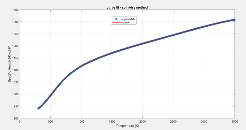
• Split wise method helps in getting a perfect fit for the original curve. The main factor in splitting the data is the 'number of splits’. More the number of splits, better the output curve.
• With the help of these methods, we can predict and manipulate the different problems and conditions for future study.

1. How to make a curve fit perfectly?

• The perfect fit is achieved when the geometric distances from the given points to the fitting curve are zero. This means that the curve fits perfectly on the points. To get a perfect fit we can increase to an order of the polynomials, this method increases the accuracy and reduces errors
• A curve fits perfectly when the values of R2">`R^2` is near to or equal to 1.
• curve passes through every data points. suitable for small No. of parameters (includes property data &calibration data)

2. How to get the best fit?

• The best fit is achieved when the geometric distances from the given points to the fitting curve are minimized, in the least-squares sense. Finding the best fit reduces the minimization of the objective function where denotes the fitting curve
• For this, we can use RMS (Root Mean square) or simple linear regression. We can change the order of polynomial to get the perfect fit. And the best way is, split the data in two or more data folds and do the curve fit.
• The curve does not pass through every point. suitable for large no. of parameters, for an overdetermine system where No. of data points are too many & not highly. accurate(error)

3.What could be done to improve the cubic fit?

• The split wise method is used for curve fit.
• This improves the curve to fit best to the data.

References:

1. http://www.math.utah.edu/~palais/pcr/spike/Evaluating the Goodness of Fit -- Fitting Data (Curve Fitting Toolbox) copy.html

2. https://projects.skill-lync.com/projects/Curve-Fitting-and-criterion-to-choose-best-fit-41860

3. https://en.wikipedia.org/wiki/Curve_fitting#Fitting_lines_and_polynomial_functions_to_data_points