Otto Cycle Visualizer in MATLAB using Engine Kinematics

AIR STANDARD CYCLE

AIM: Write a MATLAB Program that can solve an otto cycle and make plots for it.

OBJECTIVES:

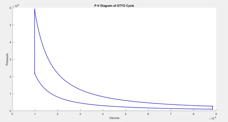
• Code should create a PV diagram.
• Should output the thermal efficiency of the engine.

THEORY:

• The cycle of the Otto engine is called the Otto cycle. It is one of the most common thermodynamic cycles found in automobile engines and describes the functioning of a typical spark ignition piston engine.
• In contrast to the Carnot cycle, the Otto cycle does not execute isothermal processes because these must be performed very slowly.
• In an ideal Otto cycle, the system executing the cycle undergoes a series of four internally reversible processes: two isentropic (reversible adiabatic) processes alternated with two isochoric processes.
• During the Otto cycle, work is done on the gas by the piston between states 1 and 2 (isentropic compression). Work is done by the gas on the piston between stages 3 and 4 (isentropic expansion). The difference between the work done by the gas and the work done on the gas is the network produced by the cycle, and it corresponds to the area enclosed by the cycle curve

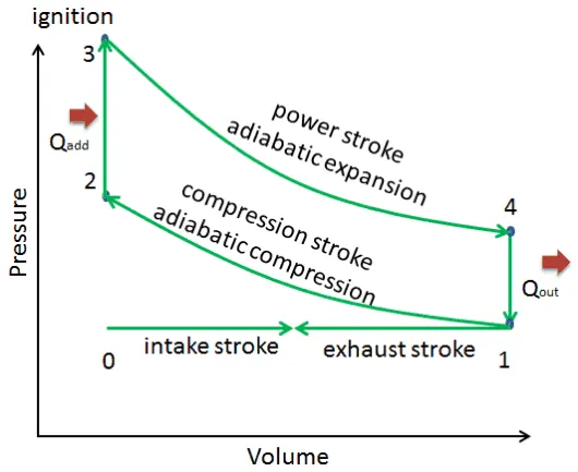
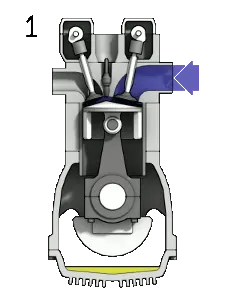
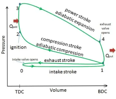
• Otto cycle is shown above on P–V diagram. The spark-ignition engine is modelled with this Otto cycle.
• The actual P-V diagram for an engine has rounded corners because of the processes of combustion take place at a finite rate.
• The Ideal Otto cycle has sharp corners because the ‘combustion’ is switched on and off instantaneously.

The Otto cycle consists of following four processes:

1. Process 1 → 2: Isentropic compression or Reversible adiabatic compression of air.
2. Process 2 → 3: Heat addition at constant volume.
3. Process 3 → 4: Isentropic expansion or Reversible adiabatic expansion of air.
4. Process 4 → 1: Heat rejection at constant volume.

• Isentropic compression (compression stroke) – The gas (fuel-air mixture) is compressed adiabatically from state 1 to state 2, as the piston moves from bottom dead centre to top dead centre. The surroundings do work on the gas, increasing its internal energy (temperature) and compressing it. On the other hand, the entropy remains unchanged. The volume changes, and the ratio (V₁ / V₂) is known as the compression ratio.
• Isochoric compression (ignition phase) – In this phase (between state 2 and state 3), there is a constant volume (the piston is at rest) heat transfer to the air from an external source while the piston is at rest at the top dead centre. This process is intended to represent the ignition of the fuel-air mixture injected into the chamber and the subsequent rapid burning.
• Isentropic expansion (power stroke) – The gas expands adiabatically from state 3 to state 4 as the piston moves from top dead centre to bottom dead centre. The gas works on the surroundings (piston) and loses an amount of internal energy equal to the work that leaves the system. Again, the entropy remains unchanged.
• Isochoric decompression (exhaust stroke) – In this phase, the cycle completes by a constant-volume process in which heat is rejected from the air while the piston is at the bottom dead centre. The working gas pressure drops instantaneously from point 4 to point 1. The exhaust valve opens at point 4.

PROCEDURE:

• Inputs of our program are,

1. Specific Heat Ratio (`γ`)= 1.4

State point 1:

1. Inlet pressure, P1 = 101325 pa
2. Inlet air temperature, T1= 500 k

State point 3:

1. Max. Temperature in compression chamber, T3 = 1900k

Engine Parameters

1. Bore = 0.5m
2. Stroke length = 0.5m
3. connecting rod length, con_rod = 0.3m
4. compression ratio, cr = 10

• After defining all our inputs, we can calculate the swept volume, clearance volume and the volume at state point 1
• After that we have to calculate all the pressure, volume and temperature of all the 4 state points
• By using governing equations, we can calculate all the state points in a p-v diagram of an otto cycle.
• Similarly, the thermal efficiency can also calculate accordingly using the formula given.
• For plotting the calculated state variables on a p-v diagram with just using plot command will yield into incorrect p-v diagram.
• So, for that, a different function needs to be created for storing different value of crank angle rotation as compression and expansion occurs in different stroke or cycle.
• This function can be called to main program and accordingly we can plot the curve from various points obtained.
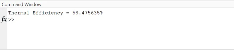
• Thermal efficiency can be obtained on the command window by using fprintf command.

GOVERNING EQUATIONS:

• Isentropic process:

`PV^γ=constant`

• Isochoric process:

`P/T=constant`

• Ideal gas equation:

`(PV)/T=constant`

• Compression Ratio

`Cr=(Vs+Vc)/(Vc)`

• Swept volume

`Vs=π/4d^2l`

• Change of Volume inside the engine combustion chamber is given by

`V/Vc=1+1/2(Cr−1)[R+1−cosθ−(R^2−sin^2θ)^(1/2)]`

• Thermal Efficiency

`η=1−(1/(Cr)^(γ−1))`

were,

P = Pressure (`Nm^2`)

V = Volume (`m^3`)

T = Temperature (Kelvin)

`γ` = ratio of specific heats

`Cr` = compression ratio

Vs = Swept Volume

Vc = Clearance Volume

V = Volume when piston moves at an angle

d = Bore

l = stroke length

a = crank pin radius = stroke length/2

R = Ratio of length of connecting rod to crank pin radius

PROGRAM:

Function code: (Separate code in a new script, save the code as the exact name of the function name in the script)

function [V] = engine_kinematics(bore,stroke,con_rod,cr,start_crank,end_crank)

         %Calculating input requirements for the Equation
         a = stroke/2;
         R = con_rod/a;

         %Calculating swept & clearance volume
         v_s = (pi/4)*bore^2*stroke;
         v_c = v_s/(cr-1);

         %assigning a array of values for theta
         theta = linspace(start_crank,end_crank,180);

         %splitting the complex equation in to 3terms
         term1 = 0.5*(cr-1);
         term2 = R+(1-cosd(theta));
         term3 = (R^2-sind(theta).^2).^0.5;

         %Calculating volume traces 
         V = (1+term1*(term2-term3)).*v_c;
end

code explanation:

• This function is defined to calculate the volume traces, while the piston moves from top dead centre to bottom dead centre and vice versa.
• we defined the function with 5 inputs Bore, stroke length, connecting rod length, compression ratio, starting and ending crank angle.
• And one output as an array of volume traces calculated by the given equation.
• The angle theta is assigned as an array of 180 values from starting crank angle to ending crank angle.
• Swept volume, clearance volume, crank pin radius, and the ratio of the length of the connecting rod to the crank pin radius 'R' are calculated in the function, which is required for the calculation of the final equation to find the volume traces.
• The values for the inputs can be assigned from the main program by calling the function and the results can be calculated.

note:

• Function must be saved as the exact name of the function name in the code
• During the Compression Process crank angle varies between theta = 180°-360°
• During the Expansion Process The crank angle varies between theta = 0°-180°

MAIN CODE:

 %program to plot P-V Diagram of an OTTO Cycle
 clear all 
 close all
 clc

 %Inputs
 gamma = 1.4;
 T3 = 1900;          %in kelvin

 %state variables at Point1
 p1 = 101325;        %in pascal
 T1 = 293;           %in kelvin
 %Engine geometric parameters
 bore = 0.1;         %in meter
 stroke = 0.1;       %in meter
 con_rod = 0.15;     %in meter
 cr = 9;
 %calculation of swept & clearance volumes
 v_s = (pi/4)*(bore^2)*stroke;
 v_c = v_s/(cr-1);
 v1 = v_s + v_c;

 %State Variables at Point 2
 v2 = v_c;
 %p2v2^gamma = p1v1^gamma
 p2 = p1*(cr^gamma);
 %p2v2/T2 = p1v1/T1 
 T2 = p2*v2*T1/(p1*v1);

 %isentropic Compression curve
 constant_c1 = p1*(v1^gamma);
 V_compression = engine_kinematics(bore,stroke,con_rod,cr,180,0);
 p_compression = constant_c1./V_compression.^gamma;


 %State Variables at Point 3
 %T3 given as input
 v3 = v2;
 %p3v3/T3 = p2v2/T2
 p3 = p2*(T3/T2);

 %Isentropic Expansion curve
 constant_c2 = p3*(v3^gamma);
 V_expansion = engine_kinematics(bore,stroke,con_rod,cr,0,180);
 p_expansion = constant_c2./(V_expansion.^gamma);

 %State Variables at Point 4
 v4 = v1;
 %p4v4^gamma = p3v3^gamma
 p4 = p3*(v3/v4)^gamma;
 %p3v3/T3 = p4v4/T4
 T4 = p4*v4*T3/(p3*v3);

 %Thermal efficiency
 Thermal_Efficiency = (1-(1/(cr^(gamma-1))))*100;
 fprintf('Thermal Efficiency = %f%%n',Thermal_Efficiency)

 %plotting P-V Diagram
 hold on
 %Plotting the 4 points
 plot(v1,p1,'*','Color','r')
 plot(v2,p2,'*','Color','r')
 plot(v3,p3,'*','Color','r')
 plot(v4,p4,'*','Color','r')
 %plotting the compression (process 1-2) and expansion (process 3-4) curves
 plot(V_compression,p_compression,'color','b','linewidth',1.5);
 plot(V_expansion,p_expansion,'color','b','linewidth',1.5);
 %plotting the process 2-3 & 4-3 ( Straight lines in pv diagram )
 plot([v2 v3],[p2 p3],'color','b','linewidth',1.5)
 plot([v4 v1],[p4 p1],'color','b','linewidth',1.5)
 %labeling the axises ang giving title to the plot
 xlabel('Volume')
 ylabel('Pressure')
 title('P-V Diagram of OTTO Cycle')

code explanation:

• Start this code by clear all, close all, clc we use these commands to clear the workspace off any previously used variables.
• Define all the inputs to the program, calculate the swept volume, clearance volume using the engine parameters.
• Using governing equations calculate the pressures, volumes and temperatures of al the state points
• By that we can get the all state points of our p-v plot.
• for plotting compression and expansion curves in pv plot we need to trace the volumes at each instant of the piston movement from TDC to BDC and BDC to TDC.
• For that we need to call the 'engine_kinematics' function that we are already created.
• For compression process the starting and ending crank angle should be 180° to 0° and for expansion process it is 0° to 180°.
• Assign the volume traces to another variable and calculate the pressure traces by the isentropic relation `PV^γ = constant`.
• After getting all the state points and calculating the pressure and volume traces in the compression and expansion processes,
• we need to calculate the Thermal efficiency of the otto cycle by the given equation, which can be printed on the command window using fprintf command.
• plot commands are used for plot the state points in red color and the pressure and volume traces in the blue color with line width of 1.5
• As the process 2 - 3 & 4 - 1 are isochoric, straight lines are plotted between the state points
• labelled the axes with proper names and titled the diagram.

Errors During programming:

1. Basic Typos and Syntax error

Error rectified by using '.' for doing operations on variable 'V_compression' which is a matrix array.

2. Errors while calculation

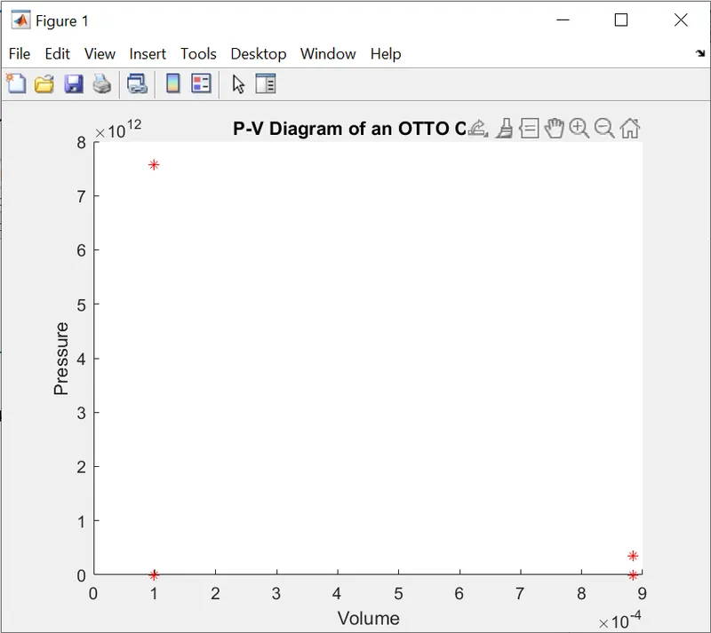
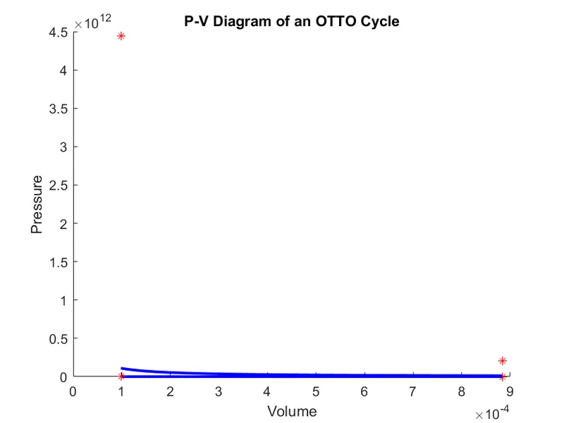
• Errors are due to the improper structure of operations which are assigned in main code as well as with in the function body.
• Errors are rectified by double checked the equations in main code and in the function code and give proper grouping for the variables in the equations with brackets '()'

OUTPUT:

1. Thermal Efficiency

2. P-V Diagram of OTTO cycle

CONCLUSION:

• The PV diagram of Otto Cycle has been plotted successfully.
• The Thermal efficiency of the Otto Cycle is 58.47%. As noted, the thermal efficiency mainly depends on compression ratio of the engine and the type of fluid. So, it can be concluded that engines with higher compression ratio will have high thermal efficiency.
• But at higher compression ratios knocking occurs, hence an optimum compression ratio must be selected.

References:

https://www.nuclear-power.com/nuclear-engineering/thermodynamics/thermodynamic-cycles/otto-cycle-otto-engine/