Finding the global maxima of stalagmite function using genetic algorithm

Genetic Algorithm

AIM: Write a code in MATLAB to optimise the stalagmite function and find the global maxima of the function.

OBJECTIVES:

• Explaining the concept of genetic algorithm and also explain the syntax for ga in MATLAB
• Plot graphs for all 3 studies and for F maximum vs no. of iteration

THEORY:

Stalagmite Function:

• Stalagmite function is the Mathematical model that actually helps us to gain Local maxima's and minima's. A stalagmite is the type of Rock formation that rises from the floor of the cave due to the accumulation of materials deposited on the floor from ceiling drippings. Stalagmite may be composed of lava, minerals, sand etc

Introduction to Optimization:

• Optimization refers to finding the values of inputs in such a way that we get the “best” output values. The definition of “best” varies from problem to problem, but in mathematical terms, it refers to maximizing or minimizing one or more objective functions, by varying the input parameters.

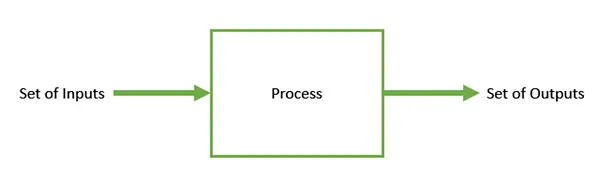
• The set of all possible solutions or values which the inputs can take make up the search space. In this search space, lies a point or a set of points which gives the optimal solution. The aim of optimization is to find that point or set of points in the search space.

Introduction to Genetic Algorithm:

• Genetic Algorithm (GA) is a search-based optimization technique based on the principles of Genetics and Natural Selection. It is frequently used to find optimal or near-optimal solutions to difficult problems which otherwise would take a lifetime to solve. It is frequently used to solve optimization problems, in research, and in machine learning.

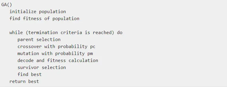
The basic structure of a GA is as follows −

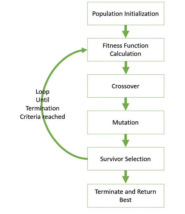
• We start with an initial population (which may be generated at random), select parents from this population for mating. Apply crossover and mutation operators on the parents to generate new off-springs. And finally, these off-springs replace the existing individuals in the population and the process repeats.
• In this way genetic algorithms try to mimic the human evolution to some extent

Phases of Genetic Algorithm:

1. Population Initialization (Coding)

• The code generates its random population of defined size and from that population the code evaluates the fitness of the members of the population according to which it forms new population based on no. of iterations performed.

There are two population models widely in use -

• Steady state: In steady state GA, we generate one or two off-springs in each iteration, and they replace one or two individuals from the population. A steady state GA is also known as Incremental GA
• Generational: In a generational model, we generate ‘n’ off-springs, where n is the population size, and the entire population is replaced by the new one at the end of the iteration.

2. Fitness Function

• It is that function which we have to optimize, and its optimization is done with the help of number of generations which have been formed by the code accordance with the fitness value of each member generated, these fitness values are used for the reproduction of the children.
• Calculation of fitness value is done repeatedly in a GA and therefore it should be sufficiently fast. A slow computation of the fitness value can adversely affect a GA and make it exceptionally slow.

3. Selection

• The selection function chooses parents for the next generation based on their scaled values from the fitness scaling function. The scaled fitness values are called the expectation values. An individual can be selected more than once as a parent, in which case it contributes its genes to more than one child

4. Creating the Next Generation

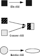
• At each step, the genetic algorithm uses the current population to create the children that make up the next generation. The algorithm selects a group of individuals in the current population, called parents, who contribute their genes—the entries of their vectors—to their children. The algorithm usually selects individuals that have better fitness values as parents

Crossover:

• Crossover is the most significant stage in the genetic algorithm. During crossover, a random point is selected while mating a pair of parents to generate offspring.

There are 3 major types of crossovers:

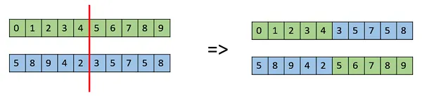
One-point crossover: In this one-point crossover, a random crossover point is selected and the tails of its two parents are swapped to get new off-springs.

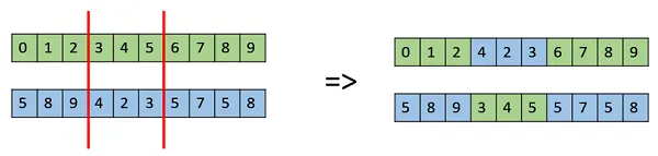
Multi point crossover: Multi point crossover is a generalization of the one-point crossover wherein alternating segments are swapped to get new off-springs.

Uniform crossover: In a uniform crossover, we don’t divide the chromosome into segments, rather we treat each gene separately. In this, we essentially flip a coin for each chromosome to decide whether or not it’ll be included in the offspring. We can also bias the coin to one parent, to have more genetic material in the child from that parent.

Mutation:

• Mutation is the part of the GA which is related to the “exploration” of the search space. It has been observed that mutation is essential to the convergence of the GA while crossover is not.
• In a few new offspring formed, some of their genes can be subjected to a mutation with a low random probability. This indicates that some of the bits in the bit chromosome can be flipped. Mutation happens to take care of diversity among the population and stop premature convergence

Bit flip mutation: In this bit flip mutation, we select one or more random bits and flip them. This is used for binary encoded GAs.

Random Resetting: Random Resetting is an extension of the bit flip for the integer representation. In this, a random value from the set of permissible values is assigned to a randomly chosen gene.

swap mutation: In swap mutation, we select two positions on the chromosome at random, and interchange the values. This is common in permutation-based encodings.

Scramble mutation: Scramble mutation is also popular with permutation representations. In this, from the entire chromosome, a subset of genes is chosen, and their values are scrambled or shuffled randomly.

inversion mutation: In inversion mutation, we select a subset of genes like in scramble mutation, but instead of shuffling the subset, we merely invert the entire string in the subset.

4. Survivor Selection:

• The Survivor Selection Policy determines which individuals are to be kicked out and which are to be kept in the next generation. It is crucial as it should ensure that the fitter individuals are not kicked out of the population, while at the same time diversity should be maintained in the population.
• In simple terms, it means the current fittest member of the population is always propagated to the next generation. Therefore, under no circumstance can the fittest member of the current population be replaced.

Syntax for GA in MATLAB:

x = ga(fun,nvars)
x = ga(fun,nvars,A,b)
x = ga(fun,nvars,A,b,Aeq,beq)
x = ga(fun,nvars,A,b,Aeq,beq,lb,ub)
x = ga(fun,nvars,A,b,[],[],lb,ub,nonlcon,IntCon,options)

fun	-	functions
nvars	-	Number of design variables
Aineq	-	A matrix for linear inequality constraints
Bineq	-	B vector for linear inequality constraints
Aeq	-	Aeq matrix for linear equality constraints
Beq	-	Beq vector for linear equality constraints
lb	-	Lower bound
ub	-	Upper bound
nonlcon	-	Nonlinear constraint function

GOVERNING EQUATIONS:

Stalagmite can be plotted as a function which is defined as,

`f(x,y)= f_(1.x)×f_(2.x)×f_(1.y)×f_(2.y)`

where,

`f_(1.x)= [sin⁡(5.1πx+0.5)]^6`

`f_(1.y)= [sin⁡(5.1πy+0.5)]^6`

`f_(2.x)=exp⁡[-4 ln⁡(2)×(x-0.0667)^2/0.64 ]`

`f_(2.y)=exp⁡[-4 ln⁡(2)×(y-0.0667)^2/0.64 ]`

PROCEDURE:

• The stalagmite function is defined separately. This function is later called into the main GA program.
• Now we define the x and y inputs using linspace command.
• Then the input vectors are transformed into array [xx,yy], so that it can be used to evaluate functions of two variables and plot three-dimensional mesh/surface plots.
• Now the values in the different matrices created can be put as an input into the function that we have created, by calling it. By this we can get the value of the stalagmite function at various values of x and y.
• Now since we have got the value of the function at various values, we now need to calculate the maxima value, which can be calculated using the ga command, which is an in-built function in MATLAB.
• Then, the total number of times the ga needs to run is defined using iteration, and with help of for loop, ga is made to run for each iteration and the value is stored in an array.
• GA generally gives the minima value (in built in MATLAB), but we need the maxima hence we can just inverse the stalagmite function by introducing a 'Negative sign'(This inverses the stalagmite curve and the Global maxima's can be found, instead minima)
• The total study time is calculated using the 'tic' and 'toc' command at the start and end of the ga for loop respectively.
• The results are then plotted using the surfc command and plot command.
• GA is made to run for 3 iterations, with each iteration having bounded inputs, unbounded inputs and increasing population size.

PROGRAM:

Function code:

function [f] = stalagmite(input_vector)

x = input_vector(1);
y = input_vector(2);

f1x = (sin(5.1*pi*x + 0.5))^6;
f1y = (sin(5.1*pi*y + 0.5))^6;

f2x = exp(-4*log(2)*((x-0.0667)^2)/0.64);
f2y = exp(-4*log(2)*((y-0.0667)^2)/0.64);

f = -(f1x*f1y*f2x*f2y);
end

code explanation:

• The stalagmite function is defined separately. This function is later called into the main GA program.
• The function defines that an input vector is assigned within the main code. Output is calculated as a stalagmite function calculated using inputs.
• Calculations are performed using the given governing equations.

Main Code:

%PROGRAM TO FIND MAXIMA USING GENEIC ALGORITHM
clear all
close all
clc

%Inpu variables
x = linspace(0,0.6,150);
y = linspace(0,0.6,150);
itration = 50;

%creating Arrays
[xx,yy] = meshgrid(x,y); 

%Loop for passing the stalagmite function
for i = 1: length(xx)
    for j = 1:length(yy)
        input_vector(1)= xx(i,j);
        input_vector(2)= yy(i,j);
        f(i,j) = stalagmite(input_vector);
    end
end

%Study1 - Unbounded Inputs 
tic
for i = 1:itration
    [inputs,fopt(i)] = ga(@stalagmite,2);
    xopt(i) = inputs(1);
    yopt(i) = inputs(2);
end
studt1_time = toc;
%plotting the function
figure(1)
subplot(2,1,1)
surf(xx,yy,-f)
xlabel('x axis')
ylabel('y axis')
zlabel('z axis')
shading interp
hold on
plot3(xopt,yopt,-fopt,'marker','o','markersize',5,'MarkerFaceColor','r')
title('Unbounded Inputs')
subplot(2,1,2)
plot(-fopt)
xlabel('Itration')
ylabel('Function maximum')


%study2 - Bounded inputs
tic
for i = 1:itration
    [inputs,fopt(i)] = ga(@stalagmite,2,[],[],[],[],[0,0],[0.1,0.1]);
    xopt(i) = inputs(1);
    yopt(i) = inputs(2);
end
studt2_time = toc;
%plotting the function
figure(2)
subplot(2,1,1)
surf(xx,yy,-f)
xlabel('x axis')
ylabel('y axis')
zlabel('z axis')
shading interp
hold on
plot3(xopt,yopt,-fopt,'marker','o','markersize',5,'MarkerFaceColor','r')
title('Bounded Inputs')
subplot(2,1,2)
plot(-fopt)
xlabel('Itration')
ylabel('Function maximum')

%study3 - Bounded Inputs with modified Population
options = optimoptions('ga');  %Stopping Conditions for the Algorithm
options = optimoptions(options,'PopulationSize',300);
tic
for i = 1:itration
    [inputs,fopt(i)] = ga(@stalagmite,2,[],[],[],[],[0;0],[1;1],[],[],options);
    xopt(i) = inputs(1);
    yopt(i) = inputs(2);
end
studt3_time = toc;
%plotting the function
figure(3)
subplot(2,1,1)
surf(xx,yy,-f)
xlabel('x axis')
ylabel('y axis')
zlabel('z axis')
shading interp
hold on
plot3(xopt,yopt,-fopt,'marker','o','markersize',5,'MarkerFaceColor','r')
title('Bounded Inputs with modified Population')
subplot(2,1,2)
plot(-fopt)
xlabel('Itration')
ylabel('Function maximum')

Code Explanation:

DEFINING WORKSPACE AND INPUTS

• Start this code by clear all, close all, clc; we use these commands to clear the workspace off any previously used variables
• Firstly, creating the mesh from the two vectors which will be acting as a search space to find the maxima of the function.
• Creating the mesh of these two vectors using the ‘mesh’ command and defining the no. of iterations to iterate the values of the optimum values of the function.
• Now calculating the values of fitness function at each point of the mesh grid formed.

STATISTICAL STUDY WITHOUT BOUNDATION (Study1)

• In this evaluating the optimum value of fitness function at each iteration and calculating it using the above-mentioned syntax in the intro part (which gives the inputs i.e., Values of x and y at which the stalagmite function is minimum)
• Then plotting it into the surf command and providing the optimum values of the function that how it is varying.
• While using surfc applying the -ve sign to the function will generate the surface upside down which will be quite good to get the maxima of the function, as it will provide positive value for the maxima using the -ve sign.
• The shading interp command is used to remove grid lines and add shading to the surf plot.
• Also using the tic and tok command to evaluate the time used for optimizing the function.

STATISTICAL STUDY WITH BOUNDATION (Study2)

• The difference over here is in providing the upper and the lower limit in the ga so that the search space is reduced with the upper and lower boundary
• And then plotting it as like the above study
• By looking at the plot, we can see that the maximum value is in the range between x = [0,0] y = [0.1,0.1], so by giving the upper limit and lower limit as this range will give the optimum values and the global maxima.
• since, bound limits and initial conditions are crucial in any optimization technique.

STATISTICAL STUDY WITH MODIFIED POPULATION (Study3)

• If the lower bond and the upper bound are difficult to find, then if we give a large rage, the function is difficult to optimize.
• So, we need to iterate the ga function for a large time with a large initial population to optimize the function.
• In this study using the ‘optimoptions’ command to increase the size of population. The benefit of that will be it will be working on the large set of numbers, and which will be led to increase the possibilities of finding the better fitness of the function.
• Its disadvantage is that it takes longer time to evaluate.

Errors while programming:

• The Errors were made which were simple syntax errors that are rectified right away with the help of the instructions in the command window.

RESULTS:

STATISTICAL STUDY WITHOUT BOUNDATION (Study1)

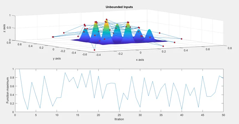
It is clear from the image above that the results are not very accurate and make a huge difference in the function optimization.

STATISTICAL STUDY WITH BOUNDATION (Study2)

• With upper boundary and lower boundary as [0,0] & [1,1]

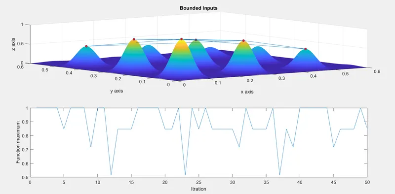
It is clear from the above figure that the variation in the optimal value of the function decreases after setting the boundary limit. Yet it is not optimal

• With upper boundary and lower boundary as [0,0] & [0.1,0.1]

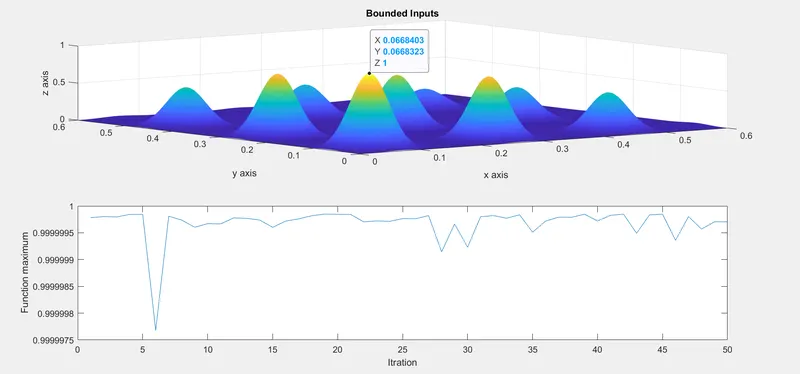
It can be much more visualized that how the best result is being displaced even with the decrease in size of population.

STATISTICAL STUDY WITH MODIFIED POPULATION (Study3)

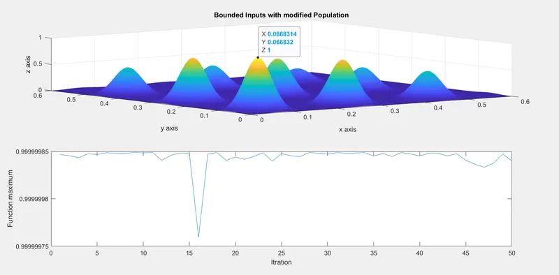
Even if the lower bond and the upper bound are difficult to find, we can optimize the function and calculate the optimum solutions.

Time study:

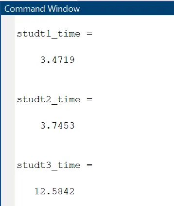
But as you can see, the optimization time will be longer as the population increases.

Workspace:

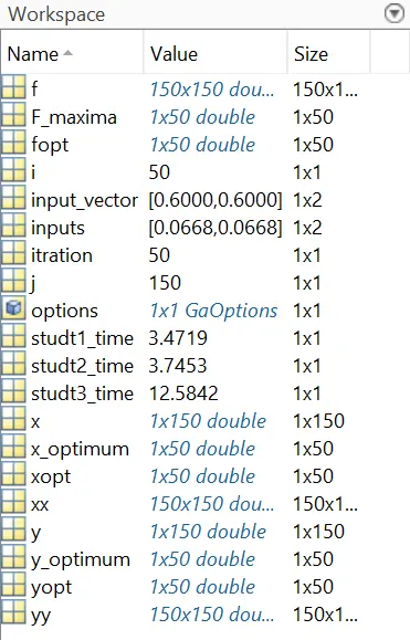
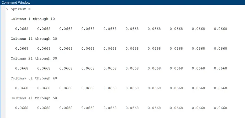
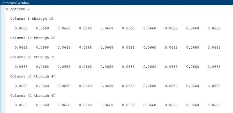
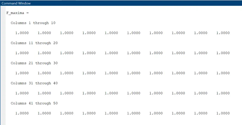
Optimum values calculated:

Optimum inputs values, x = 0.0668 & y = 0.0668

Global Maxima, F(x,y) = 1

CONCLUSION:

• Optimization of the stalagmite function is performed using genetic algorithm in MATLAB.
• Hence ga in MATLAB will only calculate the minimum value of the function, The Global maximum of a function can be found by inverting the function. Find the minimum value of the inverted function, the negative of the minimum value will give the global maximum of the function
• As no. of iteration increases probability of finding global maxima can also increases.as when population size increases with iteration, probability of global maxima can be optimised
• Bound limits and initial populations are crucial in any optimization technique, which determines the accuracy of the optimization process.

REFERENCES:

1. https://in.mathworks.com/help/gads/how-the-genetic-algorithm-works.

2. https://www.tutorialspoint.com/genetic_algorithms/index.htm

3. https://in.mathworks.com/help/gads/ga.html