MATLAB Scripting to Simulate the Rankine Cycle
Rankine cycle Simulator
AIM: Create a Rankine Cycle Simulator using MATLAB.
OBJECTIVES:
- Calculate the state points of the Rankine Cycle,
- Plot the T-s and h-s plots for the given set of inputs.
- Calculate Net work output, Back work ratio & Thermal Efficiency of Rankine cycle.
THEORY:
Rankine Cycle:
- The Rankine cycle is the archetype of all working cycles operating with steam as working fluid.
-
The Rankine cycle is the fundamental operating cycle of all thermal power plants where an operating fluid is continuously evaporated and condensed. It is the one of most common thermodynamic cycles, because in most of the places in the world the turbine is steam-driven.
-
In contrast to Carnot cycle, the Rankine cycle does not execute isothermal processes, because these must be performed very slowly. In an ideal Rankine cycle, the system executing the cycle undergoes a series of four processes: two isentropic (reversible adiabatic) processes alternated with two isobaric processes.
-
Since Carnot’s principle states that no engine can be more efficient than a reversible engine (a Carnot heat engine) operating between the same high temperature and low temperature reservoirs, a steam turbine based on the Rankine cycle must have lower efficiency than the Carnot efficiency.
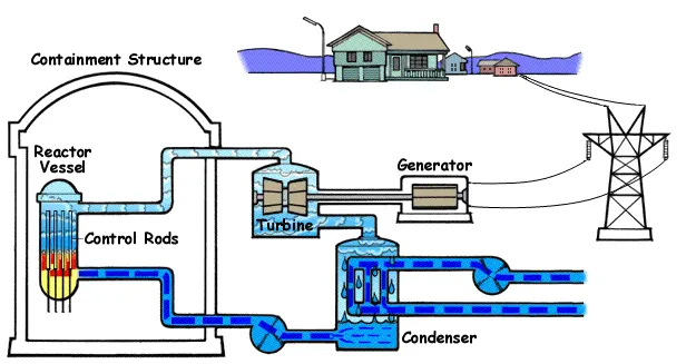
- Steam based Rankine cycles are responsible for the majority of electric power generation in the world today. The technology is readily applicable to solar thermal systems as long as the energy collected can be transported to a central power block. Water is first compressed by a feed-water pump, then boiled and superheated before being expanded through a turbine which turns an electric generator. The low-pressure steam is then condensed in a heat exchanger and fed back to the feed-water pump to be reused.
Rankine Cycle – Processes
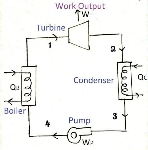
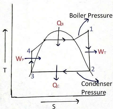
- The schematic representation of the ideal Rankine cycle and the T-s diagram of the ideal Rankine cycle are shown below,
Rankine cycle consists of four processes:
-
Process 1–2 Isentropic expansion in Turbine: The dry saturated vapour expands through a turbine, generating power. This decreases the temperature and pressure of the vapour, and some condensation may occur.
-
Process 2–3
-
Isobaric heat rejection in condenser: The wet vapour then enters a condenser, where it is condensed at a constant pressure to become a saturated liquid.
- Process 3-4
- Isentropic compression in Pump: The working fluid is pumped from low to high pressure. As the fluid is a liquid at this stage, the pump requires little input energy.
-
Process 4–1
- Isobaric heat addition in Boiler: The high-pressure liquid enters a boiler, where it is heated at constant pressure by an external heat source to become a dry saturated vapour. The input energy required can be easily calculated graphically, using an enthalpy–entropy chart (h–s chart, or Mollier diagram), or numerically, using steam tables or software.
- As can be seen, it is convenient to use enthalpy and the first law in terms of enthalpy in analysis of this thermodynamic cycle. This form of the law simplifies the description of energy transfer.
- At constant pressure, the enthalpy change equals the energy transferred from the environment through heating:
Isobaric process (Vdp = 0): `dH = dQ` → `Q = H2 – H1`
Isentropic process (dQ = 0): `dH = Vdp` → `W = H2 – H1`
Hence,
The work required for the compressor, `WPumps = H4 – H3.`
The net heat added, `Qadd = H1 – H4`
The work done by turbine, `WT = H1 – H2`
The net heat rejected, `Qre = H2 – H3`
Rankine Cycle – Ts diagram
- The temperature-entropy diagram (Ts diagram) in which the thermodynamic state is specified by a point on a graph with specific entropy (s) as the horizontal axis and absolute temperature (T) as the vertical axis.
- Ts diagrams are a useful and common tool, particularly because it helps to visualize the heat transfer during a process. For reversible (ideal) processes, the area under the T-s curve of a process is the heat transferred to the system during that process.
Thermal Efficiency of Rankine Cycle
- In general, the thermal efficiency, ηth, of any heat engine is defined as the ratio of the work it does, Wnet, to the heat input at the high temperature, Qadd.
`η = W/(Qadd)`
- The enthalpy can be made into an intensive, or specific, variable by dividing by the mass. Engineers use the specific enthalpy in thermodynamic analysis more than the enthalpy itself. It is tabulated in the steam tables along with specific volume and specific internal energy. The thermal efficiency of such simple Rankine cycle and in terms of specific enthalpies would be:
`η = 1-((h4 -h1)/(h3-h2))`
BACK WORK RATIO (BWR):
- The back work ratio is another measure of performance that is sometimes used in power plants. The back work ratio is just the fraction or percentage of the work that the turbine produces that is consumed by the pump. The lower the back work ratio, the better the performance of the power plant.
SPECIFIC STEAM CONSUMPTION (SSC):
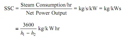
- The specific steam (or fluid) consumption is stated as the steam consumed in a power plant to generate one unit power (kW).
GOVERNING EQUATIONS:
Actual total Enthalpy, Entropy of wet steam:
`h = hf + (x*hfg)`
`S= Sf + (x*Sfg)`
where, x = Dryness fraction
`hfg = hg - hf`
`Sfg =Sg - Sf`
hf, Sf = Saturated Liquid Enthalpy & Entropy
hg, Sg = Saturated Vapour Enthalpy & Entropy
For Isentropic process,
`(T2)/(T1) = ((P2)/(P1))^(1-(1/γ)`
where, γ = `(cp)/(cv)`
Net Work Output from the Rankine cycle,
Work input (Pump),
`WPump = H4 – H3`
Work output (Turbine),
`WT = H1 – H2`
Net Work from the cycle,
`W = WT - Wpump`
Total Heat Transfer in the Rankine cycle,
Heat Addition (Boiler),
`Qadd = H1 – H4`
Heat rejection (Condenser),
`Qre = H2 – H3`
Specific Steam Consumption (SSC)
`SSC = 3600/(H1-H2)`
Back Work Ratio (BWR)
`BWR = (Wpump)/(WT)`
Thermal Efficiency,
`η = W/(Qadd)`
PROCEDURE
- Display the processes in a Rankine cycle and ask the user for the required inputs
- Problem inputs will be provided by the user.
- Standard Xsteam library is used to get the steam table data for water.
- Using XSteam Lybrary, Calculate the state points of the Rankine Cycle.
- Calculate the properties and objectives using governing equations
- Plot T-S & H-S Diagram
- Display results in the command window
PROGRAM
%Program to Simulate Rankine cycle
clear all
close all
clc
%Displaying processes in Rankine cycle
fprintf("                 RANKINE CYCLE SIMULATORn");
fprintf("n    1 - 2  is Isentropic Expansion in the Turbine ")
fprintf("n    2 - 3  is Isobaric Heat Rejection in the condenser ")
fprintf("n    3 - 4  is Isentropic Compression in the Pump ")
fprintf("n    4 - 1  is Isobaric Heat Transfer by the Boiler n")
%Assign Inputs by user
T1 = input('n Enter the Temperature at Turbine inlet [°C] = ');
p1 = input(' Enter the Pressure at Turbine inlet [bar] = ');
p2 = input(' Enter the Pressure at Condenser inlet [bar] = ');

%State point Calculation
%State Point1
h1 = XSteam('h_pT',p1,T1);
s1 = XSteam('s_pT',p1,T1);
%State Point3
p3 = p2;
h3 = XSteam('hL_p',p3);
s3 = XSteam('sL_p',p3);
T3 = XSteam('Tsat_p',p3);
%State Point2
p2;
T2 = T3;
s2 = s1;
  sf2 = XSteam('sL_p',p2);
  sg2 = XSteam('sV_p',p2);
  x2 = (s2 - sf2)/(sg2 - sf2);
  hf2 = XSteam('hL_p',p2);
  hg2 = XSteam('hV_p',p2);
h2 = hf2 + (x2*(hg2-hf2));
%State point4
p4 = p1;
s4 = s3;
 cv4 = XSteam('Cv_ps',p4,s4);
 cp4 = XSteam('Cp_ps',p4,s4);
 gamma4 = cp4/cv4;
 k = (1-(1/gamma4));
T4 = T3*((p4/p3)^k);
h4 = XSteam('h_ps',p4,s4);
%Intermediate points
%point5
p5 = p1;
hf5 = XSteam('hL_p',p5);
sf5 = XSteam('sL_p',p5);
T5 = XSteam('Tsat_p',p5);
%point6
p6 = p1;
T6 = T5;
hg6 = XSteam('hV_p',p6);
sg6 = XSteam('sV_p',p6);

%Calculations
%work output from Turbine
w_out = h1 - h2;
%Heat rejected from condenser
Q_out = h2 - h3;
%work input in pump
w_in = h4 - h3;
%Heat Addition to the boiler
Q_in = h1 - h4;
%Net Work Output
w_net = w_out - w_in;
%Back work ratio
BWR = (w_in / w_out)*100;
%Specific Steam Consumption
SSC = 3600/(h1 - h2);
%Thermal Efficiency
therm_eff = (w_net/Q_in)*100;

%Displaying Results
fprintf("nn              RESULTSnn");
%Displaying state points
fprintf(" At State Point 1: n");
fprintf("  P1 = %4.3fbar n  T1 = %4.3f°C n  h1 = %4.3fKJ/Kg n  s1 = %4.3fKJ/Kg-Knn",p1,T1,h1,s1);
fprintf(" At State Point 2: n");
fprintf("  P2 = %4.3fbar n  T2 = %4.3f°C n  h2 = %4.3fKJ/Kg n  s2 = %4.3fKJ/Kg-Knn",p2,T2,h2,s2);
fprintf(" At State Point 3: n");
fprintf("  P3 = %4.3fbar n  T3 = %4.3f°C n  h3 = %4.3fKJ/Kg n  s3 = %4.3fKJ/Kg-Knn",p3,T3,h3,s3);
fprintf(" At State Point 4: n");
fprintf("  P4 = %4.3fbar n  T4 = %4.3f°C n  h4 = %4.3fKJ/Kg n  s4 = %4.3fKJ/Kg-Knn",p4,T4,h4,s4);
%Displaying Calculations
fprintf(" Work Input (Pump Work), n   Win  = %4.3fKJ/Kg-Kn",w_in);
fprintf("n Work Output (Turbine Work), n   Wout = %4.3fKJ/Kg-Kn",w_out);
fprintf("n Net Work Output, n   Wnet = %4.3fKJ/Kg-Kn",w_net);
fprintf("n Heat Addition (Boiler), n   Qin = %4.3fKJ/Kgn",Q_in);
fprintf("n Heat Rejection (Condenser), n   Qout = %4.3fKJ/Kgn",Q_out);
fprintf("n Back work ratio, n   BWR = %f%%n",BWR);
fprintf("n Specific Steam Consumption, n   SSC = %fKg/KWhn",SSC);
fprintf("n Thermal Efficiency, n   η = %f%%n",therm_eff);

%PLOTTING T-S & H-S DIAGRAMS
%Arrays for saturation curves
T = linspace(0,400,1000);
for i = 1:length(T)
    sf(i) = XSteam('sL_T',T(i));
    sg(i) = XSteam('sV_T',T(i));
    hf(i) = XSteam('hL_T',T(i));
    hg(i) = XSteam('hV_T',T(i));
end

%T-S diagram
%saturation curve
hold on
plot(sf,T,'LineWidth',2);
plot(sg,T,'LineWidth',2);
%pressure curve
s6_1=linspace(sg6,s1,1000);
for i = 1:length(s6_1)
T6_1(i)= XSteam('T_ps',p1,s6_1(i));
end
%ploting Rankine cycle
plot([s1 s2  s3 s4 sf5 sg6 s6_1],[T1 T2  T3 T4 T5 T6 T6_1],'black','LineWidth',2);
%showing state points on the plot
text(s1,T1,'1','VerticalAlignment','bottom','HorizontalAlignment','left')
text(s2,T2,'2','VerticalAlignment','top','HorizontalAlignment','left')
text(s3,T3,'3','VerticalAlignment','top','HorizontalAlignment','right')
text(s4,T4,'4','VerticalAlignment','bottom','HorizontalAlignment','right')
legend('Saturated Liquid line','Satuated Vapour line','Rankine Cycle')
title('T-S Diagram - Rankine Cycle')
xlabel('Entropy, S [KJ/Kg-K]')
ylabel('Temperature [°C]')
grid on

%H-S Diagram
figure(2)
plot(sf,hf,'LineWidth',2);
hold on
plot(sg,hg,'LineWidth',2);
plot([s1 s2 s3 s4 sf5 sg6 s1],[h1 h2 h3 h4 hf5 hg6 h1],'black','LineWidth',2);
%showing state points on the plot
text(s1,h1,'1','VerticalAlignment','bottom','HorizontalAlignment','left')
text(s2,h2,'2','VerticalAlignment','top','HorizontalAlignment','left')
text(s3,h3,'3','VerticalAlignment','top','HorizontalAlignment','right')
text(s4,h4,'4','VerticalAlignment','bottom','HorizontalAlignment','right')
legend('Saturated Liquid line','Satuated Vapour line','Rankine Cycle')
title('H-S Diagram - Rankine Cycle')
xlabel('Entropy, S [KJ/Kg-K]')
ylabel('Enthalpy [KJ/Kg]')
grid on
Code Explanation:
- Start this code by clear all, close all, clc we use these commands to clear the workspace off any previously used variables and plots.
- For better user interaction, the cycle name and processes are displayed in the command window using the fprintf command.
- The command window calls the input for our rank cycle using the input command, the user must enter the inputs T1, p1 and p2 for our simulator.
- After getting inputs from the user, state points are calculated according to the xstream library.
- For State point 1, the inlet point of the turbine, T1 and p1 are known, and h1 & s1 are calculated using the h_pT & s_pT function in the XSteam library. State point one is not on the saturation line as the vapor may be superheated depending on the user input
- Since State Point 3 (inlet point of the pump) lies on the saturation liquid line, h3, s3 and T3 can be calculated easily using Xsteam library. p3 is equal to p2 the condenser pressure.
- For state point 2, p2 is known, T2 is equal to T3, and s2 = s1, we can calculate the vapor dryness fraction at point 2 by calculating sf & sg from the xsteam library, and we can calculate the h2 using the dryness fraction.
- For state point 4, p4 = p1 (boiler pressure), and s4 = s3, h4 can be calculated using the h_pT function in the xsteam library. Since the process is isentropic, we can use the relation (indicated in the governing equation) for the calculation of T4. For that we need to calculate cv and cp from the xsteam library
- In Process 4 - 1, the T-s and h-s diagram are not a smooth curve or line, for which intermediate points must be calculated. This can be easily calculated as it lies in the Saturation Cure.
- After calculating all the state points, we can make calculations for the net work, net heat transfer, back work ratio, specific steam comsuption and Thermal efficiecy of the Rankine using governed equations.
- The state point properties and calculated results are displayed in the command window using the fprintf command and the appropriate format specifier.
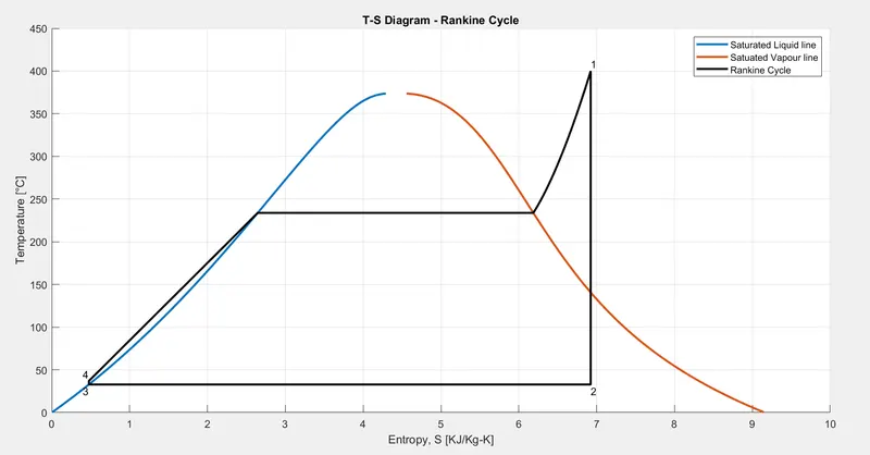
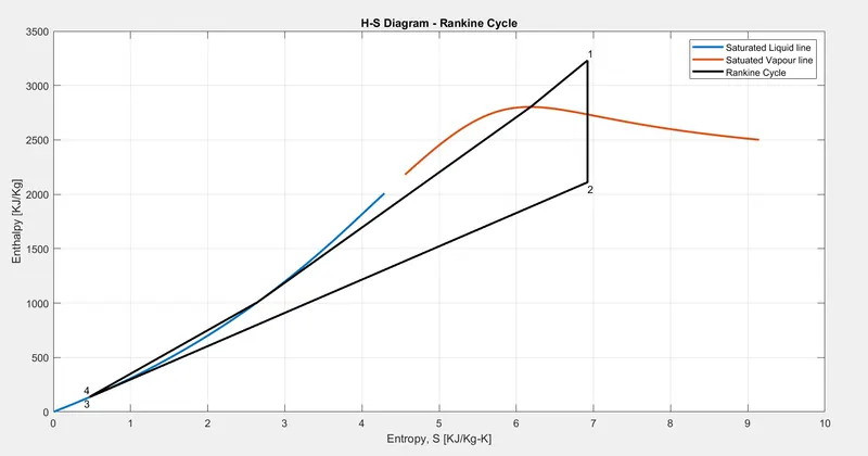
- For Plotting saturated liquid and vapour lines on both the t-s and h-s diagram a temperature array is created and the saturated liquid and vapour, enthalpy and entropy are calculated for the temperature ranges.
- For the TS diagram, plot 1 - 2 - 3 - 4 - 5 - 6 can be plotted in a straight line and 6 - 1 in a curve, for which an entropy array from s6 to s1 is created, and the temperature array is calculated using the xsteam library.
- The whole process is drawn as straight lines for the H-S diagram.
- Both diagrams are labeled, points are texted and legends are assigned.
Errors while programming:
- simple syntax errors that are rectified right away with the help of the instructions in the command window.
- Calculation errors that are fixed with proper '()' parentheses.
RESULTS
Command window:
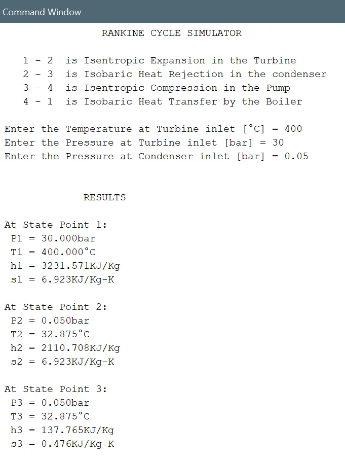
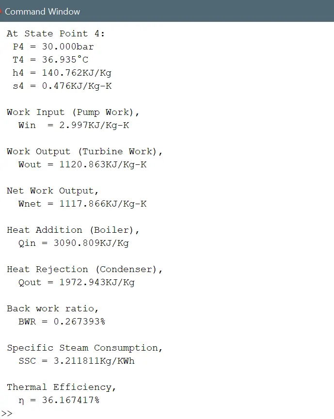
T - S Diagram
H - S Diagram
CONCLUSION
- The Rankine Cycle Simulator is created that takes input from the user, displays all state point properties and performance parameters, and plots the T-s and h-s diagram for the ranking cycle based on user inputs.
REFFERENCES:
1. https://www.youtube.com/channel/UCBa2h7ktPf1YDpOAAg2rBiA
2. https://en.wikipedia.org/wiki/Rankine_cycle#The_four_processes_in_the_Rankine_cycle
3. https://www.tlv.com/global/TI/steam-theory/wet-steam-dry-steam.html