Transient Simulation of Pendulum Using MATLAB

Solving second order ODEs

AIM: Write a program that solve second order Ordinary Differential Equation.

OBJECTIVES:

• write program to solve second order ODE of a simple pendulum with damping.
• write a program that will simulate the pendulum motion.

THEORY:

• Ordinary Differential Equations (ODEs) - An ordinary differential equation (ODE) is a differential equation containing one or more functions of one independent variable and the derivatives of those functions. The term ordinary is used in contrast with the term partial differential equation which may be with respect to more than one independent variable.
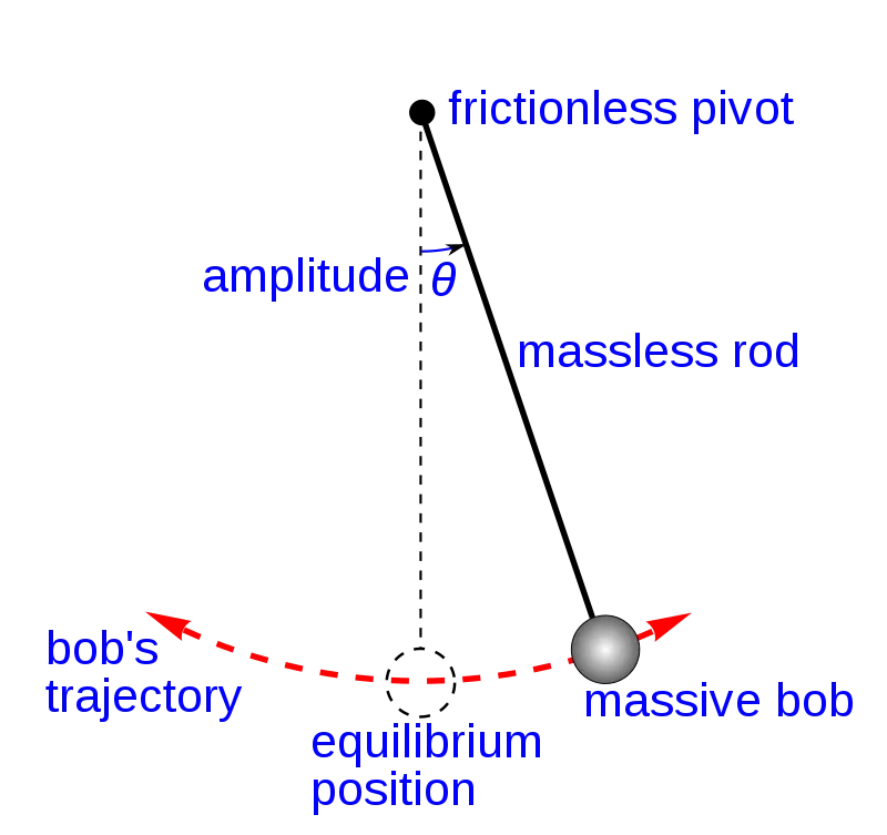
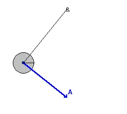
• Simple Pendulum - The simple pendulum is an idealized mathematical model of a pendulum. This is a weight (or bob) on the end of a massless cord suspended from a pivot, without friction. When given an initial push, it will swing back and forth at a constant amplitude. Real pendulums are subject to friction and air drag, so the amplitude of their swing's declines.

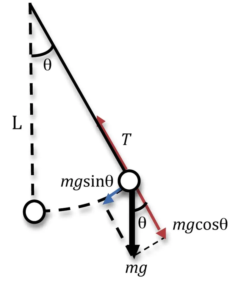
• The motion of a simple pendulum is a basic classical example of simple harmonic motion, consisting of a small bob and a massless string. Movement of the pendulum depends on the Newtons second law. When this law is written down, a second order Ordinary Differential Equation is formed that describes the position of the end of the pendulum w.r.t time.

GOVERNING EQUATIONS:

Simple pendulum with Damping:

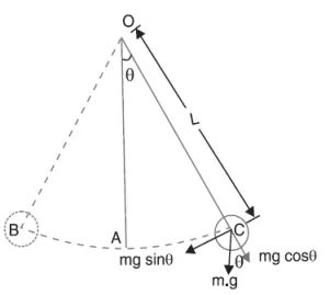
`θ` is the angle made by the movable link with vertical axis.

`L` is the length of the movable rod

`m` is the mass of bob

`b` is damping coefficient of the system.

Equation of motion of a simple pendulum with damping

`(d^2θ)/(dt^2)+b/m⋅(d(θ))/dt+g/Lsinθ=0` second order ODE -----(1)

To solve this ODE we need to reduce the order of equation into lower order

let `θ= θ1`

so this implies `(d(θ))/dt = (d(θ1))/dt = θ2` ---------(2)

therefore `(d^2θ)/(dt^2)=(d^2θ1)/dt^2=(d θ2)/dt` -----(3)

Putting the value of (2) and (3) in (1) , we get-

`(d^2θ1)/dt+b/m⋅(d(θ1))/dt+g/L⋅sinθ1=0`

therefore , `(d(θ2))/dt+b/m⋅θ2+g/L⋅sinθ1=0`

we got, `(d(θ2))/dt=−b/mθ2−g/Lsinθ1`

and, `(d(θ1))/dt = θ2`

finally,

`d/dt[(θ1),(θ2)]=[(θ2),(-(b/m)*θ2-(g/l)sinθ)]`

By solving this we get the values of `θ1 and θ2`as an array

This is how we can reduce a 2^nd order differential equation into a 1^st order differential equations

PROCEDURE:

• Inputs for our program,

Given details -

L = 1 `m`

m = 1 `kg`

b = 0.05

g = 9.81`m/s^2`

Initial conditions:

For angular displacement = 0, angular velocity=3 rad/sec at time t = 0

Simulate the motion between 0-20 sec

• Setting out the inputs for the ODE in MATLAB.
• Reduce the Higher order differential equations in to two lower order differential equations.
• Using ode45 predefined function solve the two differential equations.
• To use a ode45 solver, create a function which will return a column matrix for the solver with the reduced 1^st order equations.
• The results are stored in an array of row matrix of two columns, for the values of displacement and velocity at different time periods.
• Plot the variation of angular displacement and velocity along time.
• Generate Animation for Pendulum motion.

PROGRAM:

function code: ode_fun()

function [dtheta_dt] = ode_func(t, theta, b,g,L,m);
     
     theta1 = theta(1);
     theta2 = theta(2);

     dtheta1_dt = theta2;
     dtheta2_dt = -(b/m)*theta2 - (g/L)*sin(theta1);
     
     dtheta_dt = [dtheta1_dt ; dtheta2_dt];
end

Main program:

%Program to solve 2nd Oder ODE
clear all 
close all
clc

%Inputs
%Damping coefficient
b = 0.05;
%mass of the bob in kg
m = 1;
%gravity in m/s2
g = 9.81;
%length of the pendulum in m
L = 1;

%initial conditions
%dispacement and velocity
ini_disp_velo = [0;3];

%time points (0-20sec)
t_span = linspace(0,20,1000);

%Solve ODE
[t, results] = ode45(@(t, theta) ode_func(t, theta, b,g,L,m),t_span,ini_disp_velo);

%plotting results
figure(1)
hold on
plot(t,results(:,1));
plot(t,results(:,2));
axis([0 21 -3.5 3.5])
xlabel('time') 
ylabel('Plot')
legend('displacement','velocity')
grid on
hold off

%plotting a simple pendulum
ct=1;
for i = 1:length(t_span)
     theta = results(i,1);
     x0 = 0;
     y0 = 0;

     x1 =  L*sin(theta);
     y1 = -L*cos(theta);

     figure(2)         
     plot([x0 x1],[y0 y1],'color','b','LineWidth',2);
     hold on

     plot(x1,y1,'o','MarkerSize',30,'markerfacecolor','r');
     plot([-0.1 0.1],[0 0],'linewidth',5,'color','black');
     axis([-1.1 1.1 -1.1 0.1]);
     title('Motion of Pendulum')
     xlabel('x axis')
     ylabel('y axis')
     
     hold off
     M (ct) = getframe(gcf);
     ct = ct+1;
end

%Movie
movie(M)
videofile = VideoWriter('simple_pendulum.avi','uncompressed AVI');
open(videofile)
writeVideo(videofile,M)
close(videofile)

Code Explanation:

• Start this code by clear all, close all, clc we use these commands to clear the workspace off any previously used variables.
• Define the Input parameters g, m, b, l. and define initial conditions initial displacement and velocity.
• Define time span as an array which have time values 0 - 20sec with 1000 points between them.
• use ode45 function to solve the two differential equations.
• To use a ode45 solver, create a ode_func() which will return a column matrix for the solver with the reduced 1^st order equations.
• Provide time limits and initial conditions according to the ode45 syntax.
• The results will contain two separate columns the angular velocity and angular displacement.
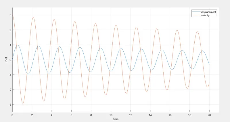
• Using the plot command angular velocities and displacements are plotted in the y-axis against time in the x-axis.
• For the simulating pendulum motion, the fixed end of the pendulum is assumed at the origin
• By using for loop, capture the variation of pendulum and plot the location of pendulum with co-ordinates varying as a function of angular displacement.
• Fix the axes, Label the axes and give titles to the plots.
• Generate the animation using movie command.
• By using video writer command, we get this movie in directory.

Errors while programming:

1. movie name already exists

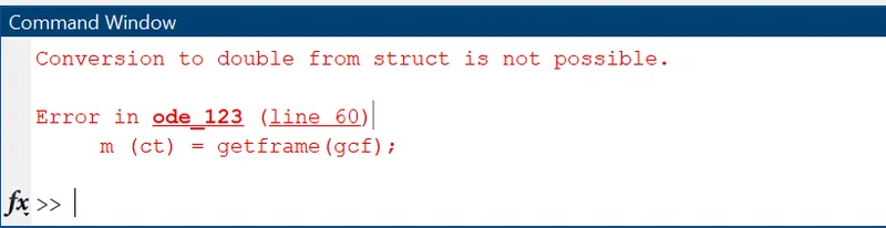
• Error rectified by assign a new variable name for getframe command.
• 'm' is an existing name for a movie, by changing it into 'M' rectified the error.

2. Error while plotting - frames overlapped

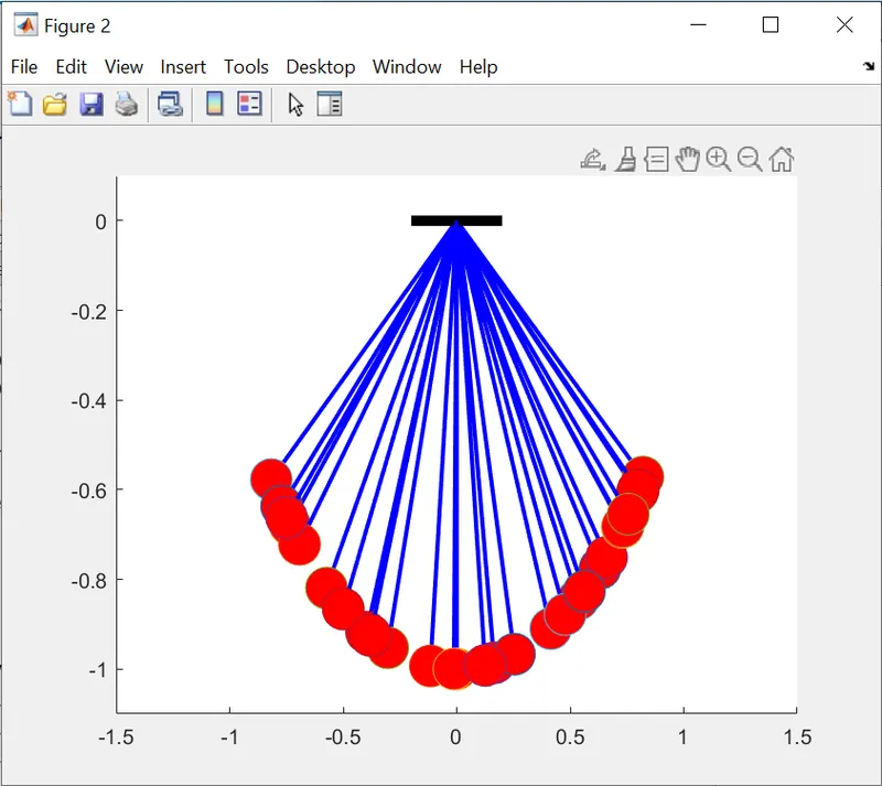
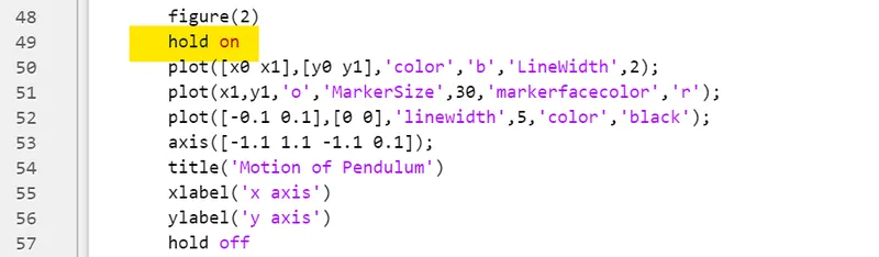
• frames overlapped while plotting and movie creation.
• Error rectified by giving hold on command after the plot command for plotting pendulum edge points.

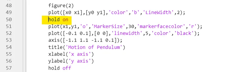
RESULTS:

1. Angular Displacement and Angular velocity of a Pendulum variation with time (0 - 20sec)

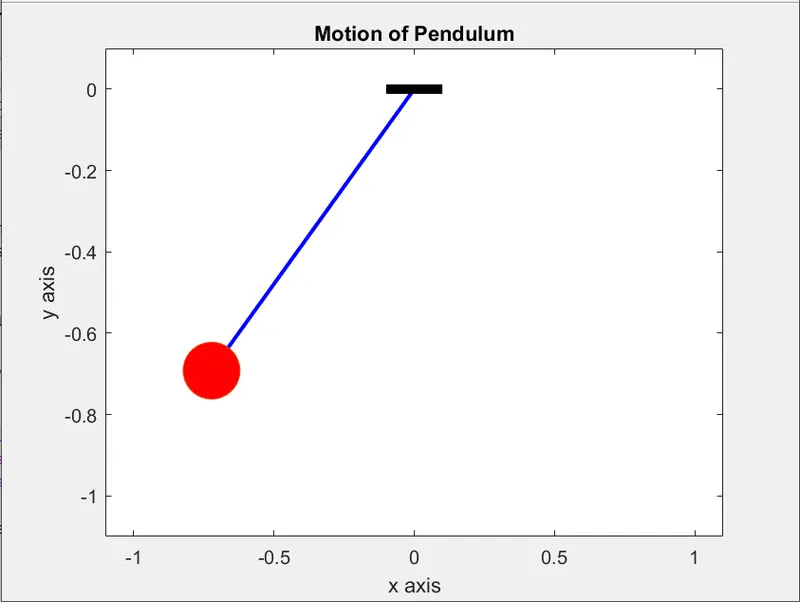
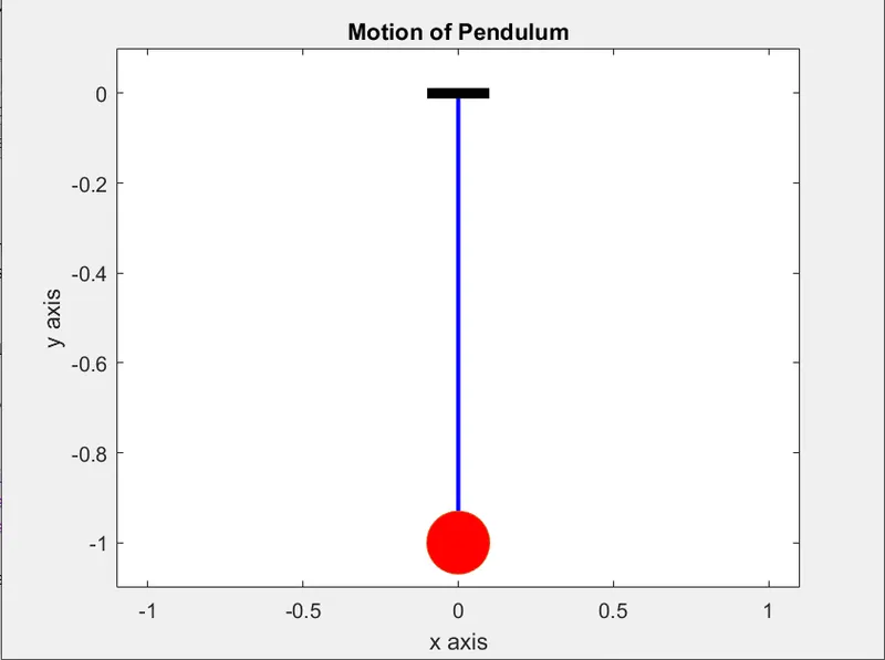
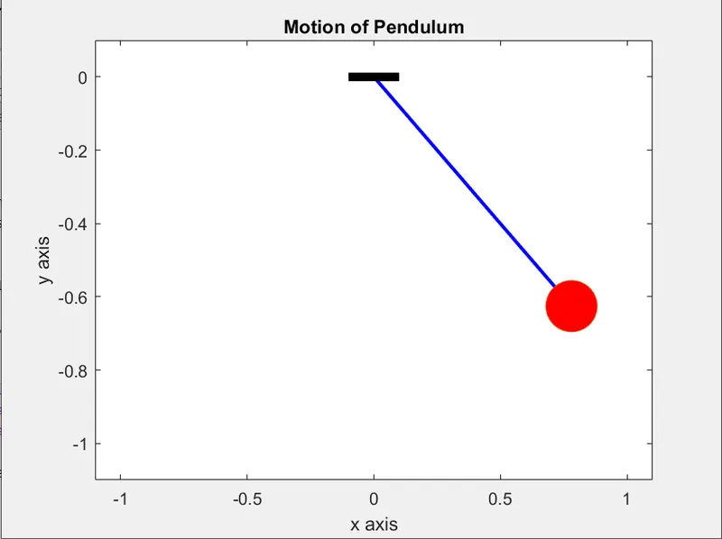
2. Pendulum motion simulation.

screenshots of the animation:

Animation video:

Link: https://youtu.be/GKvJnmSdDuI

CONCLUSION:

• Second order ODEs can be solved on MATLAB using ode45 solver inbuild function by splitting up higher order ODEs into Lower order ODEs.
• Change in Angular displacement and angular velocity with time is plotted.
• Pendulum motion is simulated successfully and made an animation video of it.