Week 4 - Curve Fitting

Aim:- To perform a curve fitting for the given dataset and to find the best fit and perfect fit for that particular using MATLAB.

Objective:-

1. To write code to fit a linear and cubic polynomial for the Specific Heat(Cp) data.
2. To plot the linear and cubic fit curves along with raw data points.
3. To study the parameters used to measure the fitness characteristics for both curves.

Theory:-

Curve Fitting

Curve Fitting is a process of constructing a curve or mathematical function, which possesses the closest proximity to the original or real series of data. By curve fitting, we can mathematically construct the functional relationship between the observed dataset and parameter values. It is a statistical technique used to drive coefficient values for equations that express the value of one (dependent) variable as a function of another (independent variable). It is highly effective in the mathematical modeling of some natural processes. By curve fitting, we can actually study and manipulate the data for different problems and different conditions.

How to fit a curve?

To fit a curve the parameter of the real dataset is a function of undefined constants of ‘n^th’ order polynomial.

• The first-degree polynomial equation,
  
  y = ax + b

is a line with slope ‘a’. A line will connect any two points, so a first-degree polynomial equation is an exact fit through any two points with distinct coordinates. It is also called an equation for the linear fit.

• If the order of the equation is increased to a second-degree polynomial, the following results,
  
  y = (ax)^2+bx+c

This will exactly fit a simple curve to three points.

• If the order of the equation is increased to a third-degree polynomial, the following is obtained,
  
  y=(ax)^3+(bx)^2+c

This is also called a cubic fit and it will fit the curve in exactly four points.

So as we increase the order of the polynomial, the nature of the curve changes accordingly.

Parameters used to measure the Fitness Characteristics :

After finding the curve which satisfies the given data points, we need to check the fitness characteristics of the curve or how well the equation is representing the data points. This can be done in 4 quantities which help us measure the goodness of fit criteria. They are,

1. The sum of squares due to error (SSE)
2. R-square
3. Adjusted R-square
4. Root mean squared error (RMSE)

1. Sum of squares due to error (SSE) – Sum of squared errors (SSE), is the sum of the squares of results or deviations predicted from actual values of data. It is a measure of the discrepancy between the data and an estimation model. A small SSE indicates a tight fit of the model to the data.
   
   SSE (sum of squared errors) = N∑i=0Error(i)^2
   

2. R-square – R-square is a statistical measure of how close the data are to the fitted regression line. R-squared is always between 0 and 1,

• 0 indicates that the model explains none of the variability of the response data around its mean.
• 1 indicates that the model explains all the variability of the response data around its mean.

In general, the higher the R-squared, the better the model fits the real data.

R2=SSRSST">R^2=SSR/SST

where,

SSR = Sum of squares of the regression

SST = SSR + SSE

3. Adjusted R-square – Adjusted R-square is a normalizing variation of R-square due to insignificant independent variables. Adjusted R-square disregards infinitesimally small increments to R-square, and only considers the variables which actually contribute to the output of the system in a drastic way.
   
   
4. Root mean squared error (RMSE) – It is an estimate of the standard deviation of the random component in the data, and is defined as,

RMSE = √(SSEn)">√(SSE/n)

Procedure/Steps

1. Before writing the code, it is important to start with clear all, close all, clc.

   clear all - removes data from the workspace,

   close all - deletes the current figure or plot,

   clc - clears all input and output from the command window.

2. Then the data of specific heat is loaded with the ‘load’ command and ‘Temperature’ as well as ‘C_p’ array is defined.
   
   
3. Then curve fitting is performed by using two functions,

• polyfit – p = polyfit (x,y,n)returns the coefficients for a polynomial p(x) of degree ‘n’ that is the best fit (in a least-squares sense) for the data in y. The coefficients in p are in descending powers, and the length of p is n+1. Here, the value on ‘n’ is 1 for linear and 3 for cubic, ‘x’ is ‘temperature’, and ‘y’ is 'cp' data. So [co_eff,S,mu] = polyfit (x,y,n) also returns mu, which is a two-element vector with centering and scaling values. mu(1) is mean(x), and mu(2) is std(x). Using these values, polyfit centers ‘x’ at zero and scales it to have a unit standard deviation. This centering and scaling transformation improves the numerical properties of both the polynomial and the fitting algorithm.

• polyval – polyval (co_eff, temperature) returns the value of a polynomial of degree ‘n’ evaluated at ‘temperature’. The input argument ‘co_eff’ is a vector of whose elements are the coefficients in descending powers of the polynomial to be evaluated. ‘polyval’ evaluates ‘co_eff’ at each element of ‘temperature’. Here polyval (co_eff, temperature,[ ], mu) is used for centering and scaling parameters of ‘mu’ which is computed by polyfit.

4. Then the curve fit data is compared with original data by plotting the curves to get linear and cubic curve fitting. The axis is shifted by using the ‘axis’ command and the legend is provided for the plot.
   
   
5. Here we are using the R-square method to evaluate the Fitness characteristics of linear and cubic curves respectively, as mentioned above.
   
   
6. M = mean(cp)returns the mean of the elements of ‘cp’ along the first array dimension.
   
   
7. The values of SSR, SSE, SST, and R-square for linear and cubic polynomial are calculated in a ‘for’ loop and the values of R-square are to be displayed on the command window.

MATLAB Code for Linear and Cubic fit

The code for linear (First Order) and Cubic (Third Order) fit is as follows,

clear all
close all
clc

% preparing the data
cp_data = load('data');
temperature = cp_data(:,1);
cp = cp_data(:,2);

% cure fit

%Linear curve fittting
%cp = a*T + b
[co_eff1,s,mu] = polyfit(temperature,cp,1);
predicted_cp1 = polyval(co_eff1,temperature,[],mu);

%Cubic Curve Fitting
% cp = a*T^2 + b*T^2 + c*T + d
[co_eff3,s,mu] = polyfit(temperature,cp,3);
predicted_cp3 = polyval(co_eff3,temperature,[],mu);

% comper my curve fitting with origianl data  
plot(temperature,cp,'linewidth',3)
hold on 
plot(temperature,predicted_cp1,'linewidth',3,'color','r')
axis([0 4000 900 1400])
xlabel('Temperature [K]')
ylabel('specific heat [kj/kmol-k]')
legend('original data','Linear Curvefit','Location','Southeast')
title('Linear Curve Fit')
grid on

figure(2)
plot(temperature,cp,'linewidth',3)
hold on
plot(temperature,predicted_cp3,'linewidth',3,'color','r')
axis([0 4000 900 1400])
xlabel('Temperature [k]')
ylabel('Specfic Heat [KJ/Kmol-k]')
legend('Original Data','Cubic Curvefit','Location','Southeast')
title('Cubic Curve Fit')
grid on

%R^2 method to find the Fitting characteristics of the Curve
M = mean(cp);

for i = 1:length(cp)
    SSR1 = sum((predicted_cp1(i)-M)^2);
    SSE1 = sum((cp(i)-predicted_cp1(i))^2);
end
SST1 = SSR1 + SSE1;
R1 = SSR1/SST1

for i = 1:length(cp)
    SSR3 = sum((predicted_cp3(i)-M)^2);
    SSE3 = sum((cp(i)-predicted_cp3(i))^2);
end
SST3 = SSR3 + SSE3;
R3 = SSR3/SST3

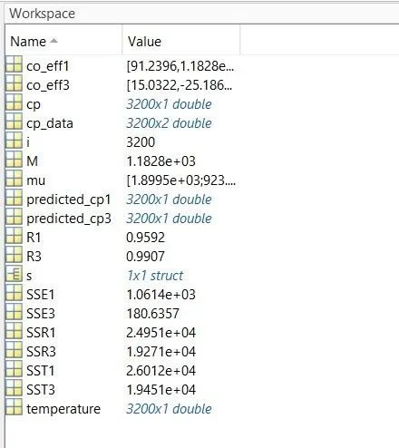
Values from Workspace

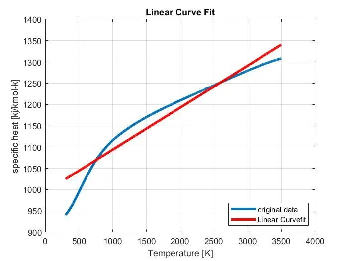
Linear Curve Fit

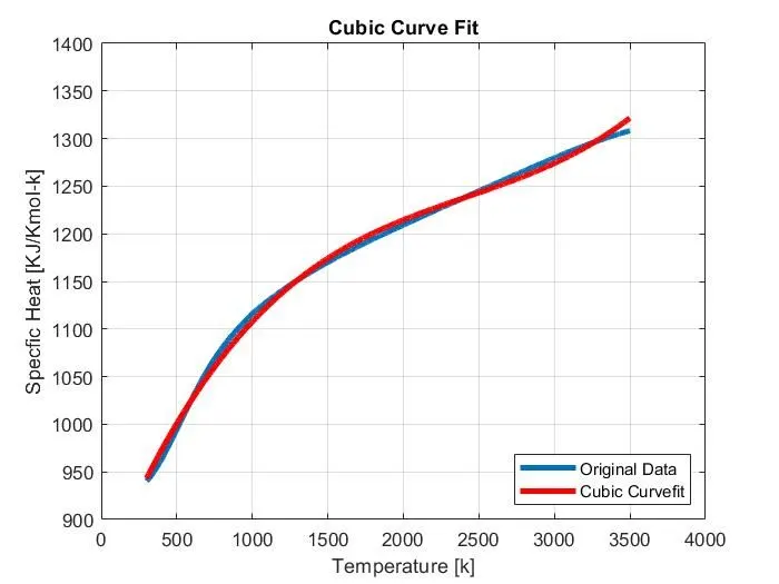
Cubic Curve Fit

RESULTS for Linear and Cubic fit :

The value of R-square for Linear fit is found to be 0.9592 and that of Cubic fit is found to be 0.9907. As we know that the higher the value of R-square, the better the fitness characteristics. Here the value of Cubic fit is higher than the value of Linear fit. So cubic curve fit has better fitness characteristics than linear curve fit. Also from both the graphs, we can see that cubic curve fit has a better resemblance to the original curve compared to linear curve fit.

An alternative way to validate Fitness Characteristics :

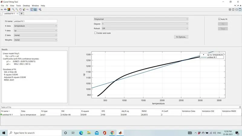
Curve Fitting Toolbox is another alternative way to validate the fitness characteristics of the curve. We just have to prepare the data first and then open the ‘Curve Fitting Toolbox’ and then select the ‘x’ and ‘y’ values. The toolbox will automatically plot the original curve. Then we have to select the degree of polynomial to fit the original curve. This will plot a new curve according to the degree of a polynomial well as will display the values of R-square, SSE, Adjusted R-square, and RMSE.

Curve Fitting Tool for Linear Curve Fit –

Curve Fitting Tool for Cubic Curve Fit

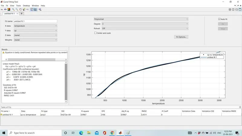
As we can see that the values of SSR, R-square, Adjusted R-square, and RMSE are displayed under “Goodness of fit” and these values are very close to the values that we found in our code.

Another alternative way to find the “Goodness of fit” is to use the following command,

[curvefit,gof,output] = fit(temperature,cp,'poly3','normalize','on')

On using this command, the values to determine “Goodness of fit” are displayed in the command window.

What could be done to improve the cubic fit?

When ‘polyfit’ and ‘polyval’ command for cubic fit is used as,

co_eff3 = polyfit(temperature,cp,3);
predicted_cp3 = polyval(co_eff3,temperature);

we get a warning as “The polynomial is badly condition”. This problem can be solved by centering and scaling the points of the curve fitting equation to get better results. Centering a variable is subtracting the mean of the variable from each data point so that the new variable's mean is 0; Scaling a variable is multiplying each data point by a constant in order to alter the range of the data. As discussed earlier, ‘mu’ which is a two-element vector with centering and scaling values is entered into the code. The comparison is shown below,

Best fit and Perfect fit:

Best fit – Best fit simply means that the differences between the actual measured values and the values predicted by the model equation are minimized. It does not mean the ‘Perfect Fit. In most cases, a least squares best fit does not go through all the points in the data set.

Perfect fit – Perfect fit means the curve should fit the original curve without showing any errors or residual values. In other words, if the R-square value of the curve is exactly 1.0000, then the curve is said to be a perfect fit. A perfect fit can be the best fit but the best fit cannot be a perfect fit. This is the basic difference between Best fit and Perfect fit.

How to get the best fit?

• To get the best fit, we should increase the degree of a polynomial of the equation and reduce the residual errors.
• By doing so, we can get values of R-square close to 1.
• As stated in the results, the best curve fit from the above program is Cubic curve fit as its value of R-square = 0.9907

How to make a curve fit perfectly?

To get a perfect fit, we need to get the value of R-square exactly equal to 1. One such solution can be the trial and error method to increase the degree of a polynomial of the equation. Using the Curve Fit Toolbox for increasing the degree of Polynomial to 8, we get a Perfect fit as shown,

But due to this, the curve fitting equation becomes more complex as there is 9 number of constants to be determined.

Another way to achieve a perfect fit is to split the data into equal sets and then plot the curve. This is also called as splitwise method, where we split the data of specific heat (C_p) and its corresponding temperature values and we will execute the program with the same order of polynomial for each data set.

Program to Split the data and plot curve fitting

%Program to Split the data and plot the curve.
clear all
close all
clc

%Data Preparation
cp_data = load('data');
temperature  = cp_data(:,1);
cp = cp_data(:,2);

%Data Splitting
temperature1  = cp_data(1:400,1);
cp1 = cp_data(1:400,2);

temperature2  = cp_data(401:800,1);
cp2 = cp_data(401:800,2);

temperature3  = cp_data(801:1200,1);
cp3 = cp_data(801:1200,2);

temperature4  = cp_data(1201:1600,1);
cp4 = cp_data(1201:1600,2);

temperature5  = cp_data(1601:2000,1);
cp5 = cp_data(1601:2000,2);

temperature6  = cp_data(2001:2400,1);
cp6 = cp_data(2001:2400,2);

temperature7  = cp_data(2401:2800,1);
cp7 = cp_data(2401:2800,2);

temperature8  = cp_data(2801:3200,1);
cp8 = cp_data(2801:3200,2);

%Cubic Fit with Centering and Scaling
[co_eff1,S,mu] = polyfit(temperature1,cp1,3);
predicted_cp1 = polyval(co_eff1,temperature1,[],mu);

[co_eff2,S,mu] = polyfit(temperature2,cp2,3);
predicted_cp2 = polyval(co_eff2,temperature2,[],mu);

[co_eff3,S,mu] = polyfit(temperature3,cp3,3);
predicted_cp3 = polyval(co_eff3,temperature3,[],mu);

[co_eff4,S,mu] = polyfit(temperature4,cp4,3);
predicted_cp4 = polyval(co_eff4,temperature4,[],mu);

[co_eff5,S,mu] = polyfit(temperature5,cp5,3);
predicted_cp5 = polyval(co_eff5,temperature5,[],mu);

[co_eff6,S,mu] = polyfit(temperature6,cp6,3);
predicted_cp6 = polyval(co_eff6,temperature6,[],mu);

[co_eff7,S,mu] = polyfit(temperature7,cp7,3);
predicted_cp7 = polyval(co_eff7,temperature7,[],mu);

[co_eff8,S,mu] = polyfit(temperature8,cp8,3);
predicted_cp8 = polyval(co_eff8,temperature8,[],mu);

%Compare curve fit with the original data
plot(temperature,cp,'linewidth',3,'color','b')
hold on
plot(temperature1,predicted_cp1,'linewidth',3,'color','r')
hold on
plot(temperature2,predicted_cp2,'linewidth',3,'color','r')
hold on
plot(temperature3,predicted_cp3,'linewidth',3,'color','r')
hold on
plot(temperature4,predicted_cp4,'linewidth',3,'color','r')
hold on
plot(temperature5,predicted_cp5,'linewidth',3,'color','r')
hold on
plot(temperature6,predicted_cp6,'linewidth',3,'color','r')
hold on
plot(temperature7,predicted_cp7,'linewidth',3,'color','r')
hold on
plot(temperature8,predicted_cp8,'linewidth',3,'color','r')
axis([0 4000 900 1400])
xlabel('Temperature [K]')
ylabel('Specific Heat [KJ/Kmol-K]')
legend('Original Data','Splitwise data Curvefit','Location','Southeast')
title('Cubic Curve Fit with Splitted Data')
grid on

Here in this code, we have the 'cp' data into 8 equal data sets and for each data set we have assumed the degree of a polynomial as '3'.

Program Output

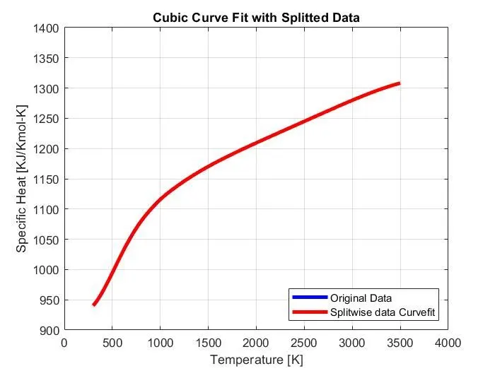
From the above curve plot, we can say that the curve for 'Original data' is not visible as the 'Splitwise data Curvfit' has perfectly fitted the original curve.

Conclusion

• From this report, we can state that there are different ways to perform Curve Fitting.
• We need to have high order polynomial equations to achieve the best fit. The higher the order of the polynomial, the better is the curve.
• The splitwise method helps in getting a perfect fit for the original curve. The main factor in splitting the data is the “number of splits’. More the number of splits, the better the output curve.
• With the help of these methods, we can predict and manipulate the different problems and conditions for future study

References

• https://in.mathworks.com/help/matlab/ref/polyfit.html?s_tid=srchtitle
• https://in.mathworks.com/help/matlab/ref/polyval.html
• https://in.mathworks.com/help/ident/ref/goodnessoffit.html
• https://in.mathworks.com/help/curvefit/evaluating-goodness-of-fit.html