Flow over Bicycle

Aim:- To write a MATLAB program to calculate Drag force against a bicycle and study the relation between-

1. Velocity and Drag Force
2. Drag co-efficient and Drag Force

Objective :-

1. To calculate the drag force on a bicycle at varying speeds.
2. A program to plot Velocity vs Drag force.
3. A program to plot Drag co-efficient vs Drag force.

Theory:-

• Drag Force - The force related to the resistance of an object as it moves through a fluid is called drag force. A Drag force acts opposite to the direction of the oncoming flow velocity. The magnitude of drag force mainly depends on-

1. The types of the surrounding fluid.
2. The shape of the object.
3. The velocity of the object.

Figure.01 Drag force

The expression of Drag Force Fd is :-

Fd = 1/2 ρAV^2Cd

Where

Fd = Drag Force (kgm/s^2);

ρ = Density of the fluid (kg/m^3);

A = Frontal Area (m^2);

V = Velocity of object (m/s);

Cd = Drag Co-efficient (unitless);

• Frontal Area (A) - Fontal Area is the area of the object which is subjected to fluid force. This area is considered 2D geometry. The total resistance offered by the vehicle is the product of the frontal area and drag coefficient.
• Drag Co-efficient - The drag coefficient is used to quantify the drag or resistance of an object in a fluid environment. it is a dimensionless quantity. it as different values for different shapes. Drag coefficient manily6 depends on Frontal Area and others factors which include the density of a fluid, the velocity of the object, etc.

Figure.02 Drag coefficient for different shape

Solution #01:-

• Program to calculate Drag Force on bicycle and study relation between Velocity and Drag Force by Plotting graph.

Programming language - MATLAB

1. Before writing the code, it's important to start with clear all, close all, clc.

   clear all - removes data from the workspace,

   close all - deletes the current figure or plot,

   clc - clears all input and output from the command window.

2. Defined all the inputs values
   • The value of Area (A) m^2 = 0.1,
   • The value of density (rho) kg/m^3 = 1.2
   • The value of velocity (v) m/s = linspace(1,5,10)
   • The value of Drag coefficient = 0.8
3. To plot the velocity vs drag force, the coefficient of drag force value is kept as constant the velocity is varied use linspace.
4. The accursed value of velocities and drag forces are plot on a graph using the plot command.
5. The x-axis and y-axis are labeled respectively using the xlabel and ylabel command.

MATLAB Coding

% A program to calucate the drag force for bicycle 
% plot Velocity vs Drag Force 

clear all
close all
clc

%inputs
%Drag coefficient
c_d = 0.8

%Area m^2
A = 0.1

%Density kg/m^3
rho = 1.2

% velocity m/s
v = [1 2 3 4 5];

drag_force = 0.5*rho*A*v.^2*c_d

plot(v, drag_force)
xlabel('velocity (m/s)')
ylabel('Drag Force (N)')
title('Velocity vs Drag Force') 
grid on

Output:-

• All the calculated values are given below (figure.03)

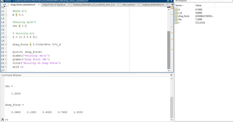
Figure.03

• The plot between Velocity vs Drag Force is given below,(Figure.04)

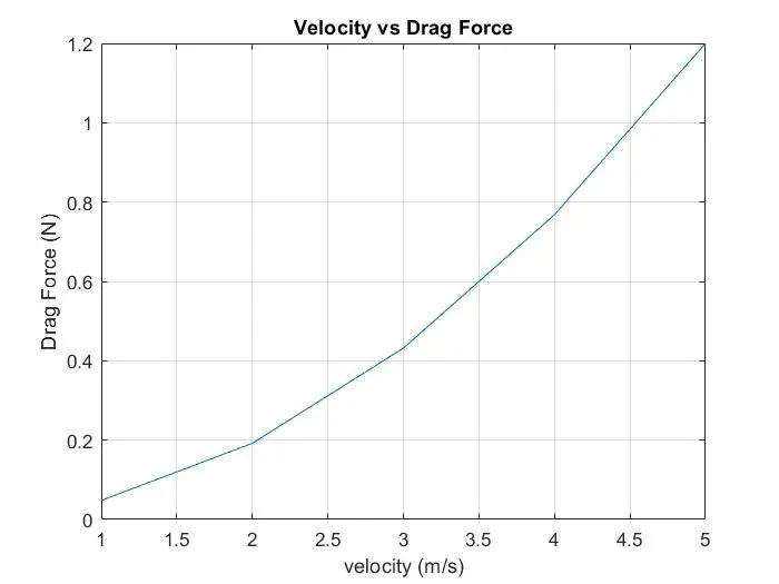
Figure.04 Velocity vs Drag Force

Solution #02:-

• Program to calculate Drag Force on bicycle and study relation between Drag Co-efficient and Drag Force by Plotting graph.

Programming language - MATLAB

1. Before writing the code, it's important to start with clear all, close all, clc.

   clear all - removes data from the workspace,

   close all - deletes the current figure or plot,

   clc - clears all input and output from the command window.

2. Defined all the inputs values
   • The value of Area (A) m^2 = [0.375 0.370 0.339 0.425 0.468];
   • The value of density (rho) kg/m^3 = 1.2
   • The value of velocity (v) m/s = 7
   • The value of Drag coefficient c_d= [0.625 0.633 0.654 0.655 0.678];
3. To plot the drag coefficient vs drag force, the velocity is kept as constant the Drag force value is varied use linspace.
4. The accursed value of drag coefficient and drag forces are plot on a graph using the plot command.
5. The x-axis and y-axis are labeled respectively using the xlabel and ylabel command.

MATLAB Coding

% A program to calucate the drag force for bicycle 
% plot Drag Co-efficient vs Drag Force 

clear all
close all
clc

%inputs
%Drag coefficient
c_d = [0.625 0.633 0.654 0.655 0.678];

%Area m^2
A = [0.375 0.370 0.339 0.425 0.468];

%Density kg/m^3
rho = 1.2;

% velocity m/s
v = 7;

F_d = 0.5*rho*A.*c_d*v^2;

plot(A.*c_d, F_d)
xlabel('Drag co-efficient')
ylabel('Drag Force (N)')
title('Drag co-efficient vs Drag Force') 
grid on

Output:-

• The plot between Drag co-efficient vs drag force is given below in figure.05

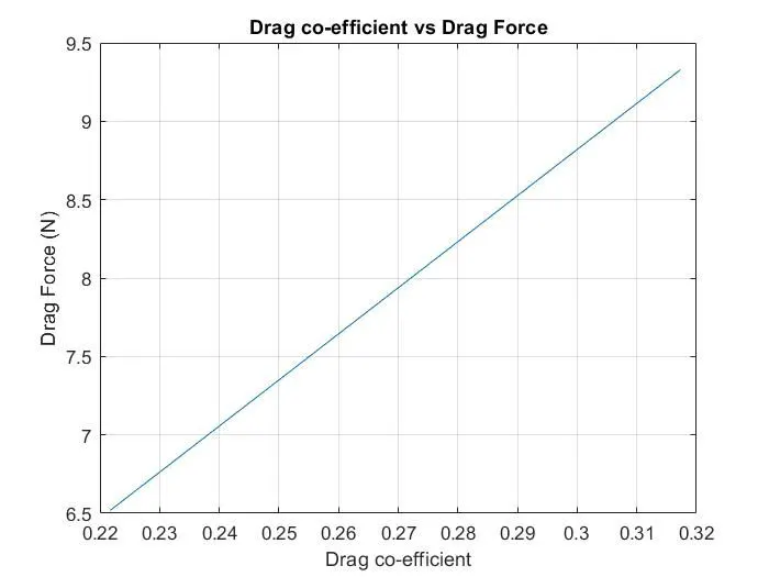
Figure.05 Drag co-efficient vs Drag force

Result based on graph

Drag force increases linearly with Drag co-efficient. Every value of drag co-efficient efficient is associated with a particular value of a frontal area.

References:-

• https://dc.uwm.edu/cgi/viewcontent.cgi?article=1031&context=etd
• https://link.springer.com/article/10.1007/s12283-017-0234-1