Week 3 - Solving second order ODEs
Aim:- To solve an ordinary differential equation (ODE) and use the calculated information to animate the motion of the pendulum in MATLAB.
Objective:-
- To write a program to simulate the transient behavior of a simple pendulum.
- To create an animation of the motion of a simple pendulum using MATLAB.
Theory:-
Ordinary Differential Equation (ODE)
In mathematics, an ordinary differential equation (ODE) is a differential equation containing one or more functions of one independent variable and the derivatives of those functions. An ordinary differential equation (ODE) is an equation that involves some ordinary derivatives (as opposed to partial derivatives) of a function. The term ordinary is used in contrast with the term partial differential equation which may be with respect to more than one independent variable. The differential equations are classified as Linear, Non-linear, Homogenous, and Non-Homogenous equations. Based on the order of equation, they are also classified as First Order Ordinary Differential Equation, Second Order Ordinary Differential Equation, or ‘nth’ Order Equation. In engineering, ODE is used to describe the transient behavior of a system and one of its examples is a simple pendulum.
Simple Pendulum
A simple pendulum is defined to have an object that has a small mass, also known as the pendulum bob, which is suspended from a light wire or string, as shown in the figure below.
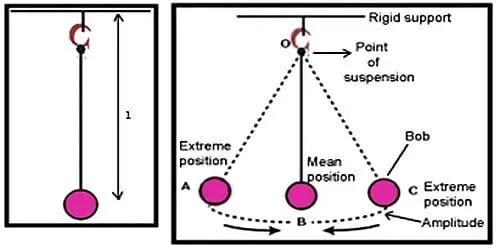
The dynamic behavior of the pendulum bob is important to understand the motion of the simple pendulum. When the pendulum bob is given an initial push while it is at rest, it experiences a force sideways. It is displaced from its equilibrium position and starts to oscillate about the pivot point swinging back and forth. In general, the motion of a simple pendulum is considered to be simple harmonic motion with constant amplitude and is given by the equation,
Where,
θ = Angular displacement of the pendulum bob;
g = Acceleration due to gravity in m/s^2;
l = length of the pendulum in m.
b = damping coefficient;
m = mass of the pendulum bob kg.
The differential equation is of order '2' and this is called a second-order Ordinary differential equation (ODE) for a simple pendulum. by using this equation we can simulate the transient behavior of a simple pendulum using MATLAB.
Derivation for code simplification
Let angular displacement θ=θ1 and angular velocity will b,
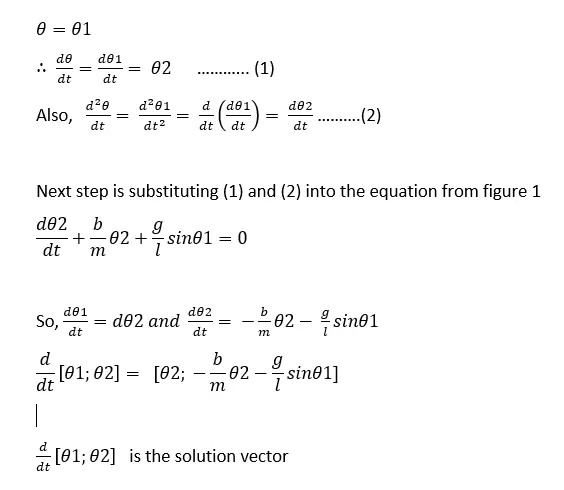
Where,
θ1 = Angular Displacement of the pendulum bob;
θ2 = Angular Velocity of the pendulum bob;
Procedure/Steps
- Before writing the code, it is important to start with clear all, close all, clc.
clear all - removes data from the workspace,
close all - deletes the current figure or plot,
clc - clears all input and output from the command window.
- The given input values of b, g, l,and m are entered and the initial condition for angular displacement 'θ1θ1' = 0, angular velocity 'θ2θ2' = 3 rad/sec are entered to the variable ‘theta_0’.
- The time span of the motion of simple pendulum ‘t_span’ is taken to be 10 seconds with 500 equal intervals.
- To establish the relationship between all the input values in second-order ODE, a different function code is written which is as follows,
Function,
> The function code is based on the matrix which we derived. here the first value of the LHS row matrix is defined as 'theta' and the second value is defined as 'theta2'.function [dtheta_dt] = ode_func(t,theta,b,g,l,m); theta1 = theta (1); theta2 = theta (2); dtheta1_dt = theta2; dtheta2_dt = -(b/m)*theta2-(g/l)*sin(theta1); dtheta_dt = [dtheta1_dt ; dtheta2_dt] end
>Then all the corresponding equations and relations are entered.This function is named as 'ode_func'. - [t, results] contains the results which we need to plot with respect to time in which 'results(1)' contains angular displacement values in radian and 'results(2)' contains angular velocity values in radian. By using this we can calculate different values of angular displacement and angular velocity with respect to time. Thus ‘results’ is an array.
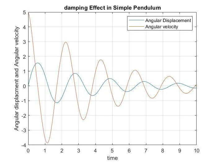
- Using these results, the graph of angular displacement and angular velocity with respect to time is plotted.
- Then counter ‘ct’ is initialized. Here ‘ct’ is a variable that simply increments by a specific step value in every iteration of a loop.
- To provide continuous motion to the pendulum, a ‘for’ loop is used where all the values of ‘t_span’ are assigned to a variable ‘i’ one at a time. The coordinates of the points of the line (x_start, y_start, x_end, y_end) and their corresponding relations are entered to form the link or string of the pendulum. This line and its motion are thus plotted using a suitable axis.
- The ‘marker’ command is used to form a circle or the bob of the pendulum and the counter is incremented by 1.
- The ‘pause’ command is used to achieve better animation speed.
- Then ‘getframe’ command is used to capture the motion of the lines and stored in a variable M.
- By using the ‘movie’ command, Matlab is going to make a movie with all the frames stored in variable M
- To save this movie, the ‘videofile’ command is used which has the option to store the video in an Uncompressed ‘avi’ format along with the file name.
- Then the video file is opened after the plot, the movie is run and after completion, the video stops or closes.
MATLAB Coding:-
clear all
close all
clc

b = 0.05;
g = 9.81;
l = 1;
m = 0.1;

% intial condition
theta_0 = [0;5];

% time point
t_span = linspace(0,10,500);

% solve ODE
[t, results] = ode45(@(t,theta) ode_func(t,theta,b,g,l,m),t_span,theta_0);

plot(t, results(:,1));
hold on
plot(t, results (:,2));
ylabel ('Angular displacment and Angular velocity');
xlabel ('time');
grid on
title('damping Effect in Simple Pendulum');
legend('Angular Displacement','Angular velocity');


%For loop
% Before stsrting the for loop, a counter value was define

ct=1;
for i = 1:length(results(:,1))
    x_start = 0
    y_start = 0
    x_end = l*sin(results(i,1))
    y_end = -l*cos(results(i,1))

    %plotting the animation
    figure(2)
    plot ([-1 1], [0 0], 'linewidth',5)
    hold on
    plot([x_end x_start], [y_end y_start], 'linewidth',3)
    hold on

    plot(x_end,y_end,'o','markersize',20,'markerFacecolor','y')
    title('Animation of transient behaviour of a pendulum')
    axis([-1.5 1.5 -1.5 1.5])
    pause(0.03)
    hold off

    M(ct) = getframe(gcf)
    ct = ct+1
end

% Animation of the pendulum

movie(M)
videofile = VideoWriter('pendulum Animation.avi','uncompressed avi')
open(videofile)
writeVideo(videofile,M)
close(videofile)
Program Output:-
ANIMATION:
Error faced while programming:
- Error in movie M(ct)
Solution:- The counter 'ct' must be incremented after the M(ct) = getframe(gcf) command. if the counter is incremented before, then the movie will contain initialized frames.
References:-