Week - 4 - Crash Box Simulation

INTRODUCTION:

Crash box is a thin-walled component which deforms axially and absorbs the energy during impact. The crash box is widely used in automobile and aerospace industry to absorb accidental impact energy. This safety component reduces the injuries by accidents and provides more safety to the passengers. Basically the kinetic energy is absorbed and reduced evenly by the crash box.

The given crash box is a simple rectangular channel-shaped component. The objective of the task is to simulate the crash test for a given crash box and find the stress, strain, acceleration and energy plots. Crash box of thickness 1.2mm and 1.5mm are compared keeping all other parameters same.

GEOMETRY:

The given geometry is shown in fig 1.1 below. It is a simple rectangular channel which can be thought of as the most simple crash box.

                     

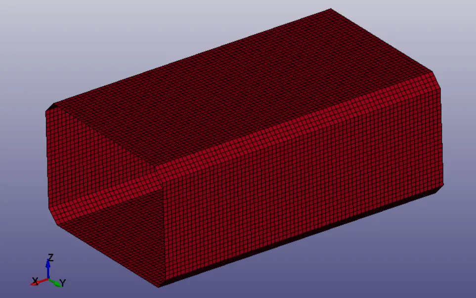
                                                                  Fig 1.1 Given crash box geometry

The given component is meshed with shell elements. The crash box is meshed with 9656 number of shells are with 9792 number of total nodes.

PROCEDURE:

The step by step procedure for a complete simulation setup is discussed below.

The given input file is of .k file format, this file can be opened through LS-PrePost by selecting it as a keyword file. The unit system used for the analysis is gm-mm-ms. The given file does not consist of any rigid wall so a new rigid wall is created by using *RIGIDWALL_PLANAR card. This is done by selecting create entity>RigidWall>create option. The rigidwall type is selected as planar. N1-N2 method is selected which helps in selecting two nodes and normal for the generated rigidwall. The rigid wall is offset by 10mm from the crash box.

 

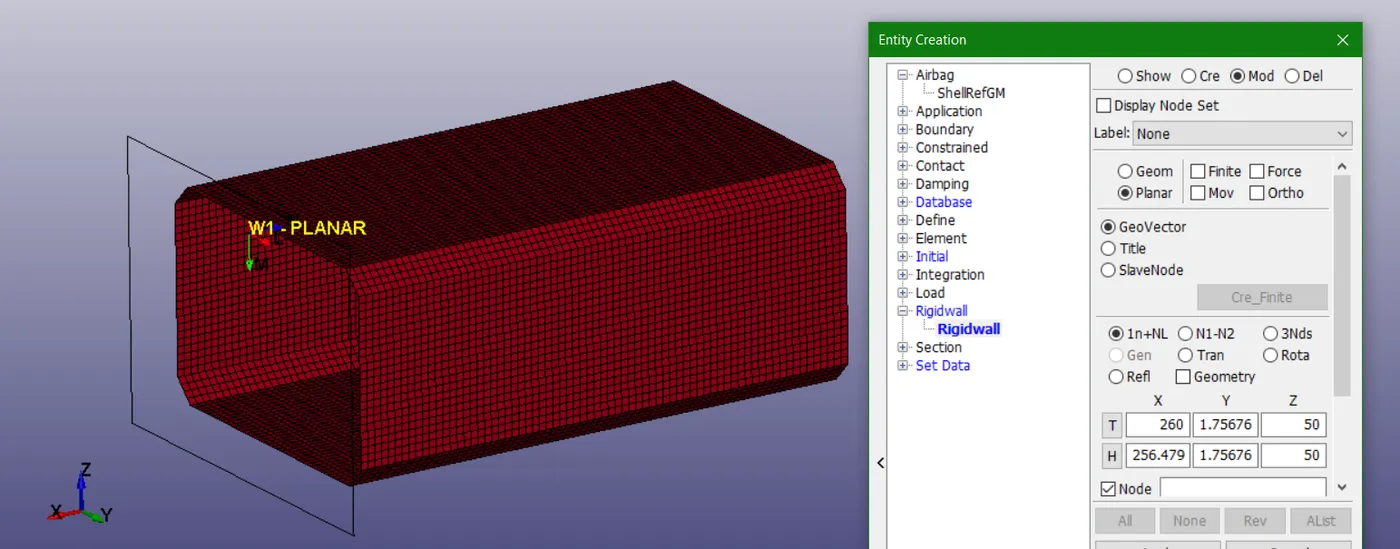
                                         Fig 1.2: Rigidwall created with create entity option

The direction of the normal of the generated rigidwall and the velocity should be in the opposite direction. This replicates the correct physics of crash. If the direction of normal of rigidwall and velocity of the crashbox is same then the crashbox penetrates through the rigidwall which is unacceptable. The black border in the fig 1.2 and fig 1.3 shows the rigid wall location.

         

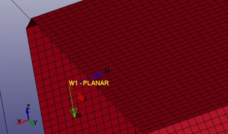
                           Fig 1.3: Direction of normal of rigidwall depicted by blue colour line

Now, the section properties for the crash box are defined by using *SECTION_SHELL card. Only the shell thickness value of 1.2mm is defined keeping all other parameter values as default. One more card with new section ID is defined and the shell thickness 1.5mm is assigned to it.

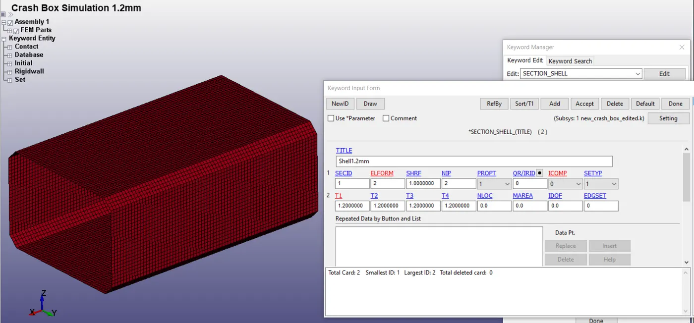
                               Fig 1.4: Shell thickness assignment by using *SECTION_SHELL card

After this, material is defined to the crash box. The crash box undergoes large deformation which are above elastic limits. So a plasticity model ‘Piecewise linear plasticity’ is used to define the crash box. Crash box is assumed to be made of steel. The following properties are defined in the material card:

Massdensity(RO)=0.00785gmmm3">Massdensity(RO)=0.00785gmmm3Massdensity(RO)=0.00785gmmm3

Young′sModu̲s(E)=2.1⋅105gmmmms2">Young'sModu––s(E)=2.1⋅105gmmmms2Young′sModu̲s(E)=2.1⋅105gmmmms2

Poisson′sratio(PR)=0.3">Poisson'sratio(PR)=0.3Poisson′sratio(PR)=0.3

Yieldstress(SIGY)=310gm(mmms)2">Yieldstress(SIGY)=310gm(mmms)2Yieldstress(SIGY)=310gm(mmms)2

tan≥ntModu̲s(ETAN)=2100gmmmms2">tan≥ntModu––s(ETAN)=2100gmmmms2tan≥ntModu̲s(ETAN)=2100gmmmms2

The other material properties in the card are kept to the default values. The tangent modulus is the slope of the stress-strain curve and is taken as 1% of Young’s modulus from the literature study.

 

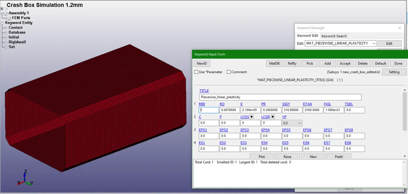
             Fig 1.5: Material property definition by *MAT_PIECEWISE_LINEAR_PLASTICITY card

Define velocity to the crash box by using create entity option. The selection is done by part and the whole crash box geometry is assigned a velocity of 13.889mm/ms (50Kmph). This velocity is assigned to each node of the selected part that is carsh box here. The fig 1.6 shows the velocity assignment and fig 1.7 shows the card generated after the initial velocity assignment card.

 

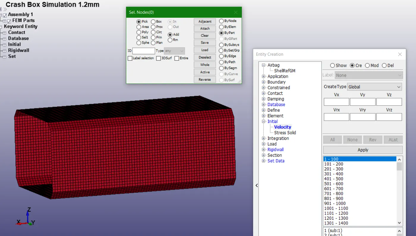
                                                Fig 1.6: Creating initial velocity entity

 

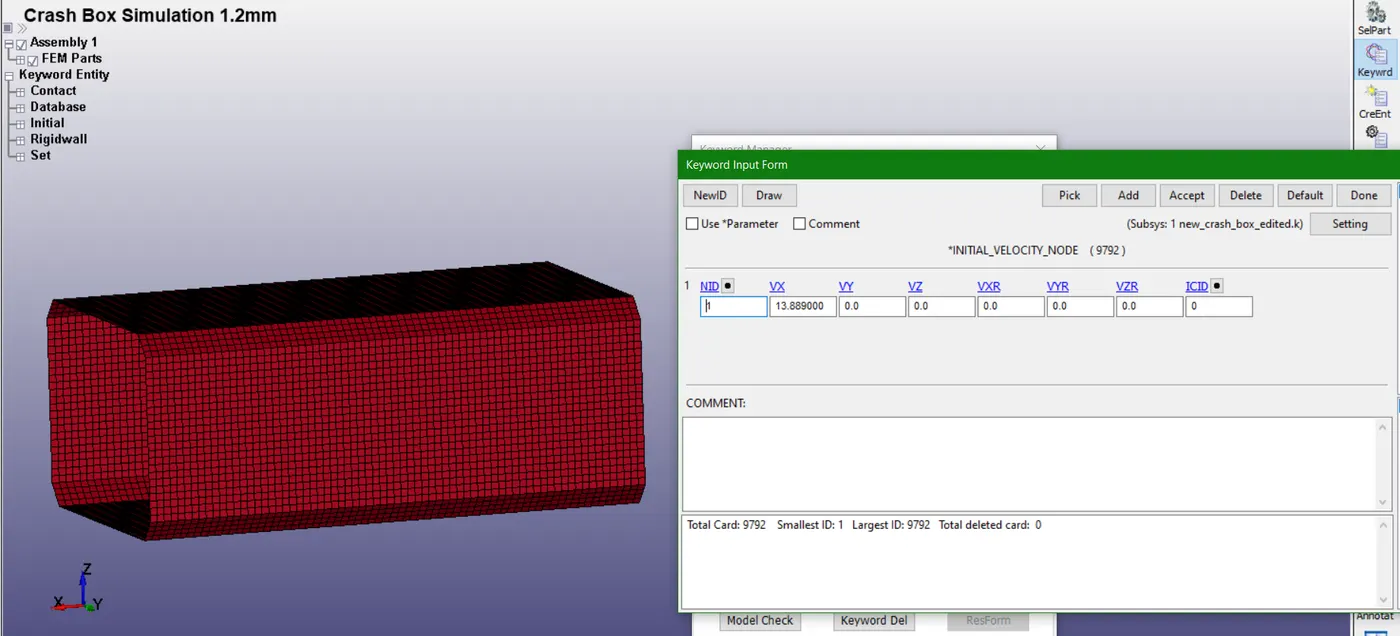
                                                Fig 1.7: *INITIAL_VELOCITY_NODE card

Then assign the created section properties and material properties to the part (crash box). This is done by updating *PART card.

 

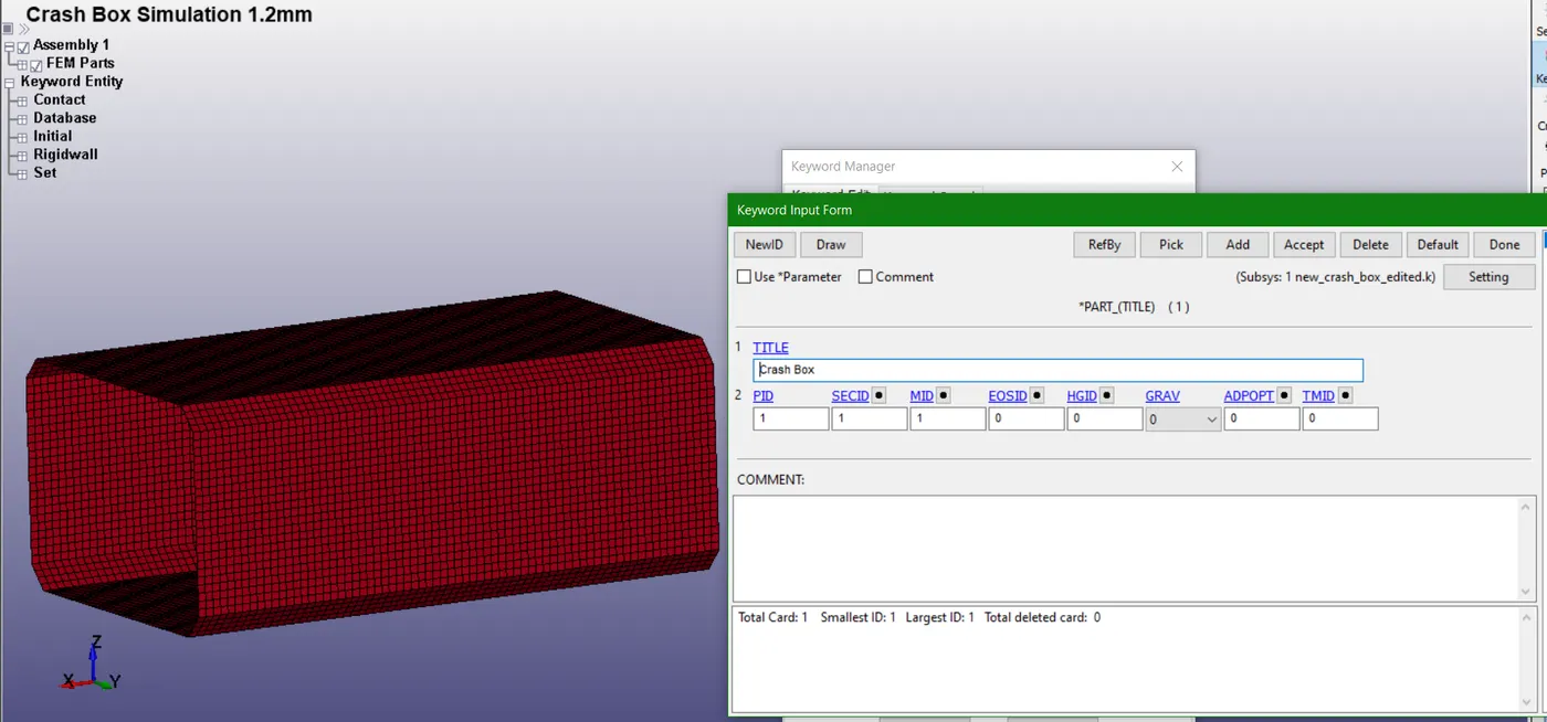
                 Fig 1.8: Defining section properties and material properties to the part(crash box)

Contact definition is an important aspect, the specific contact type used for this analysis is an automatic single surface. This algorithm sets up contact when a surface of one body contacts with itself or the external surface of other body. This algorithm searches the surfaces for contact automatically. Here there is no need to define a master surface so only slave surface definition is sufficient.

 

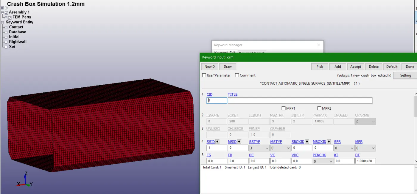
                        Fig 1.9: Contact definition using an automatic single surface contact type

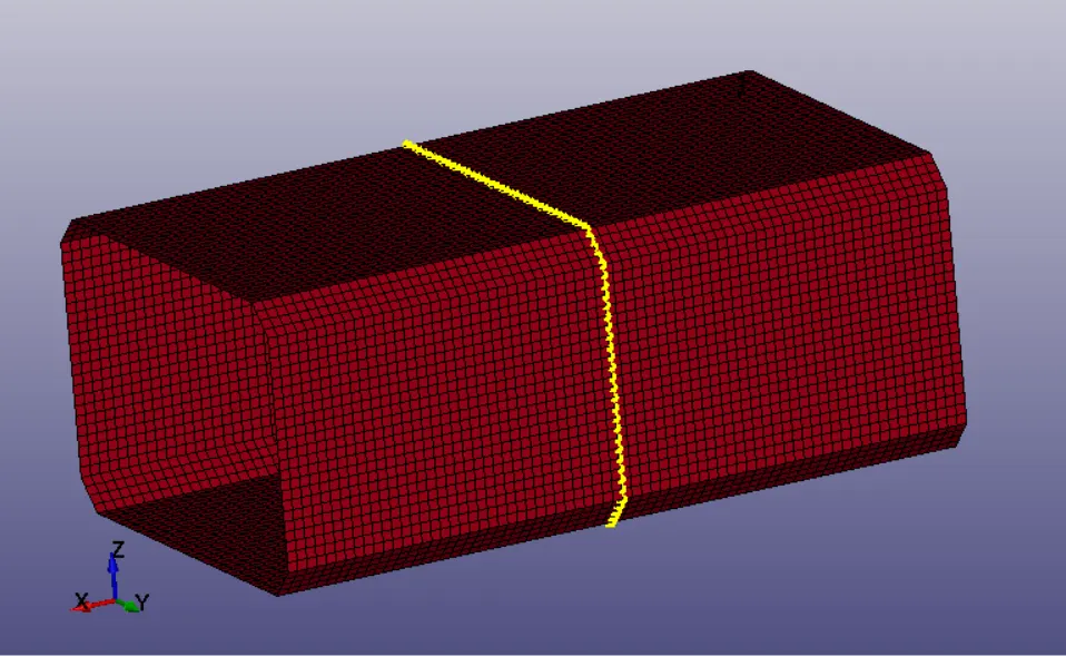
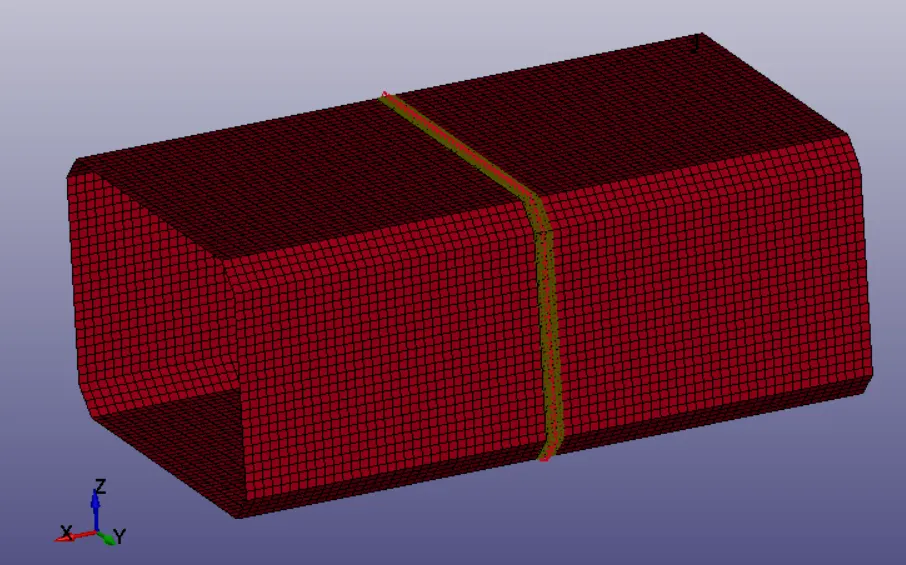
In this analysis, we need the stress, strain, acceleration and energy values at nodes, sections and over the whole body. For generating section forces, creating specific node list and element list which defines the desired section is necessary. Mode list and element list can be created by 'create entity' option and selecting the required nodes and elements. The fig 1.10 – 1.11 shows the node and element selection. The selection of nodes and elements are done by picking each node and element through create entity>set data>*SET_NODE/*SET_SHELL toolbox.

   

                                          a)                                                                                  b)

Fig 1.10: Nodes (a) and elements (b) selected in node/element list option for extracting section forces

Termination time is assigned by using *CONTROL_TERMINATION card, *CONTROL_ENERGY is also used to calculate the energy dissipation. Hourglass energy, rigidwall energy, sliding interface energy can be calculated by this card assignment. Termination (end time) is calculated analytically by using the distance between rigidwall and crash box (10mm) and velocity of the crash box (13.889mm/ms). The calculated time is 0.7199ms but additional time is considered to simulate the crashing and bouncing back/buckling and folding of the crash box. So, the total time 1ms is assigned as end time in the *CONTROL_TERMINATION card.

Now, the output data is generated by using *DATABASE card. Database cards like BINARY_D3PLOT, ASCII_option (ELOUT-element data, GLSTAT-global statistics and energies, MATSUM-part energies, NODOUT-nodal motions, RCFORC-resultant contact interface forces, SLEOUT-contact interface energies etc) are assigned for generating output data. For getting the acceleration plot of a node in the middle of the crash box, element selection is necessary. This is done picking the desired elements by using *DATABASE_HISTORY_NODE card. For generating section forces *DATABASE_CROSS_SECTION_SET card is used and the nodes and shell elements from the fig 1.10 are assigned for node-set ID (NSID) and shell element set ID (SSID) respectively. This card basically defines the cross-section for resultant forces written in ASCII file SECFORC.

   

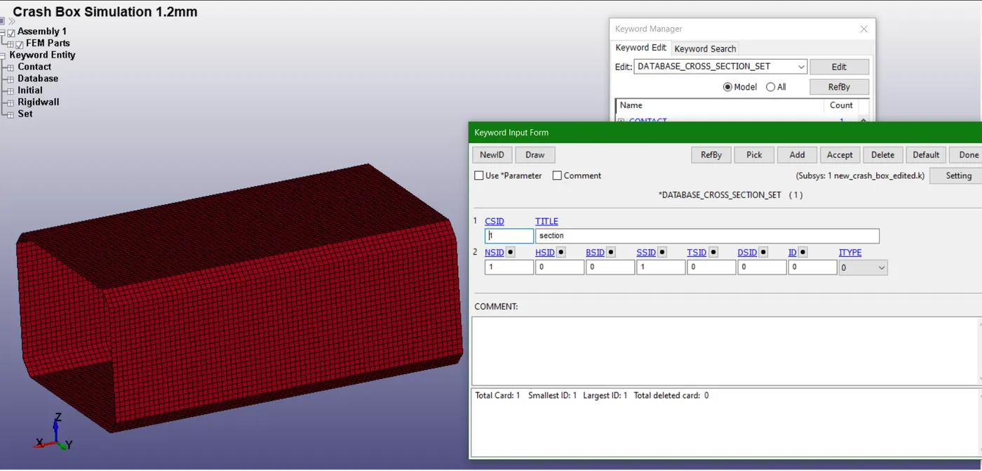
                          Fig 1.11: Defining cross-section properties to generate section forces

After this all card assignments the model is ready for simulation. The keyword file is saved with other name and saved in the folder. This same keyword file is opened through LS-DYNA manager which solves the problem by reading the keyword file step by step.

RESULTS AND DISCUSSION:

BINARY_D3PLOT card gives the binary output for the entire model. This basically gives the animation of the deformed geometry. Various other output parameters are evaluated and are discussed in the following section.

Cross-section forces in the middle of the crash box:

    

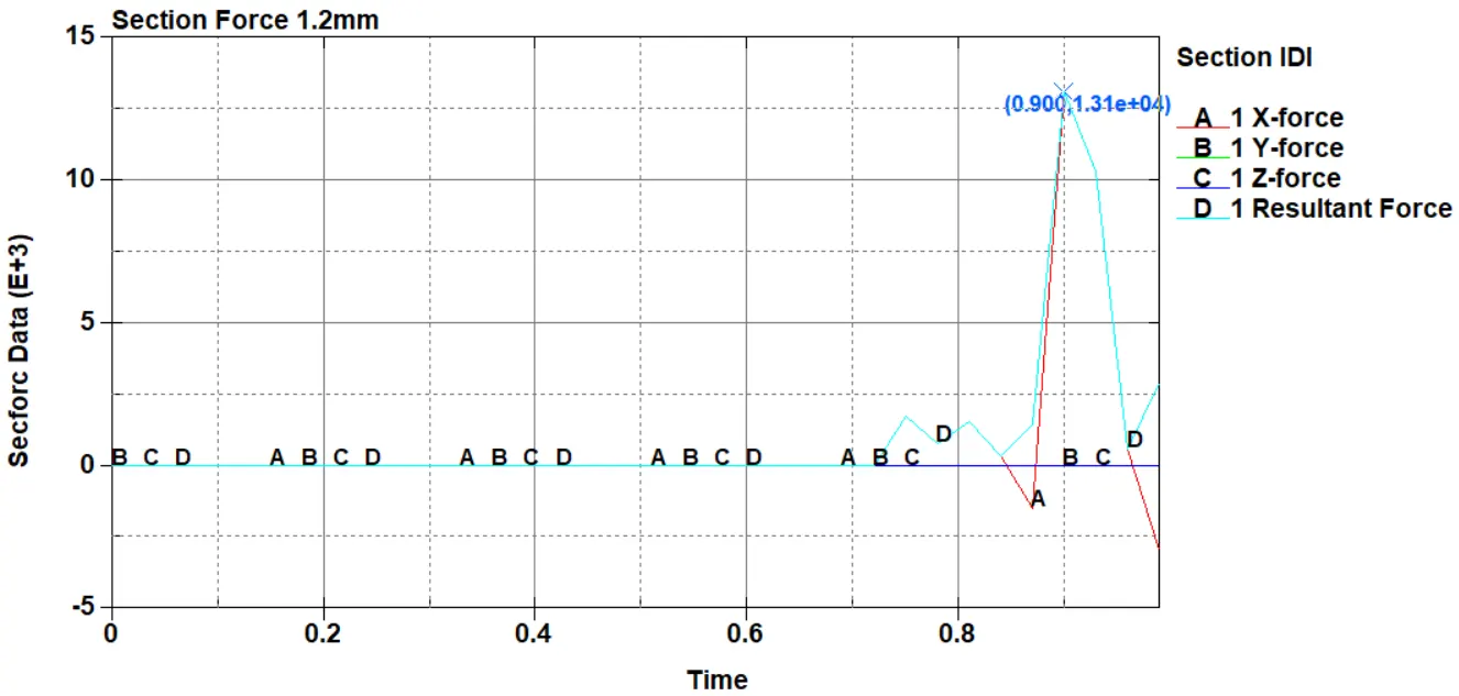
Fig 1.12: Cross-section forces in X, Y and Z direction along with resultant force for 1.2mm shell thickness

 

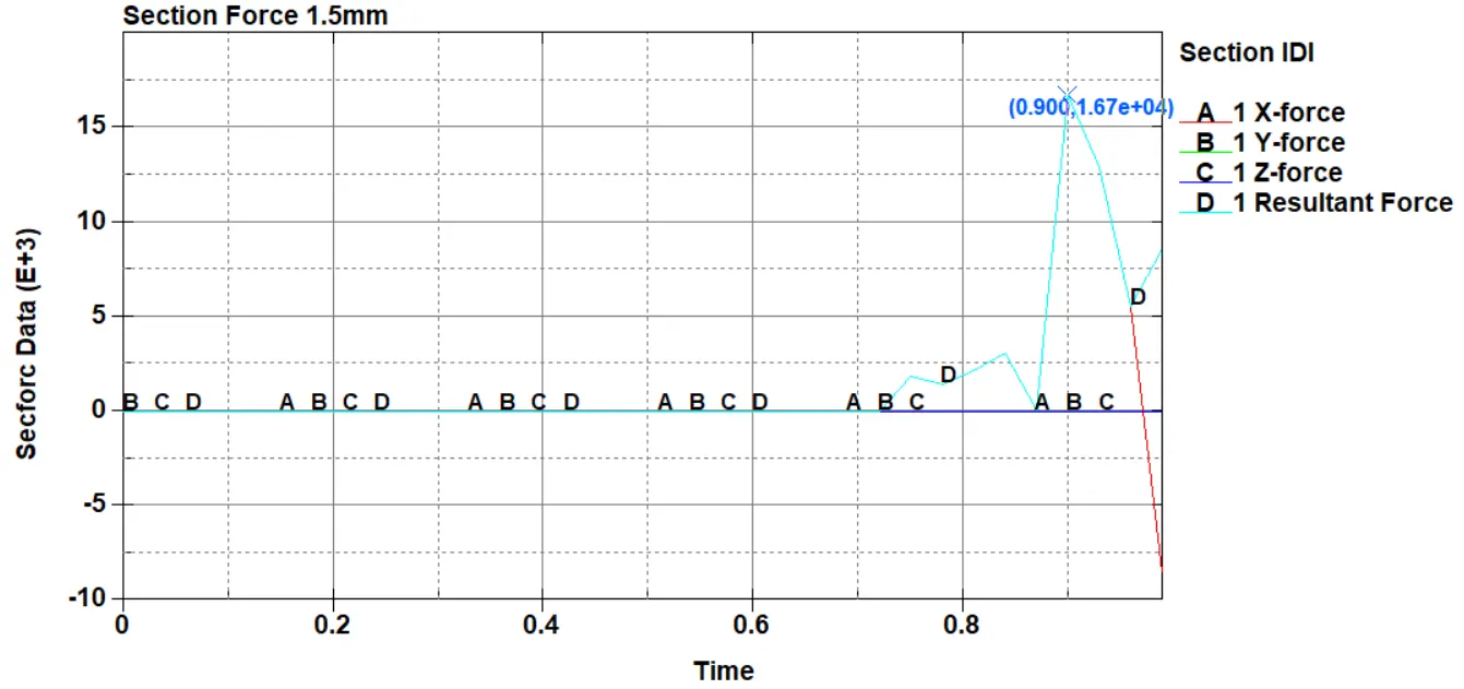
Fig 1.13: Cross-section forces in X, Y and Z direction along with resultant force for 1.5mm shell thickness

Figure 1.12 and 1.13 shows lower force values for the Y and Z direction. This is because the crash box has the velocity along X-axis and impacts the rigidwall in that direction. The force value peaks during the impact and then dropdowns after the crash box bounces back. Resultant force for both shell thicknesses is almost equal to X-direction section force. It can be clearly seen in figure 1.12 and 1.13 that resultant force values generated in the crash box for 1.5mm shell thickness are higher (16.7⋅103gmmmms2">16.7⋅103gmmmms216.7⋅103gmmmms2 ) than 1.2mm shell thickness (13.1⋅103gmmmms2">13.1⋅103gmmmms213.1⋅103gmmmms2). This is because the 1.5mm shell thickness crash box has extra mass compared to 1.2mm shell thickness with the same acceleration values in both the cases. So the extra mass is responsible for producing extra force values at the same acceleration.

Acceleration plot of a node in the middle of the crash box:

 

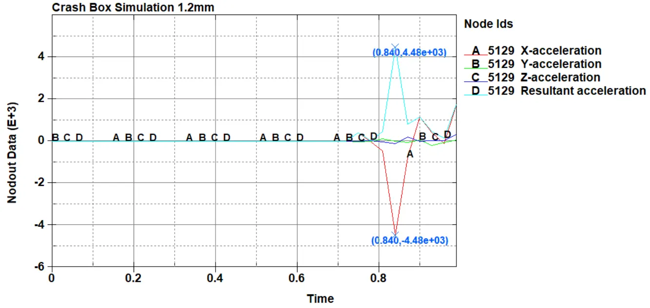
Fig 1.14: Nodal acceleration of a node selected in the middle of the crash box for 1.2mm shell thickness

 

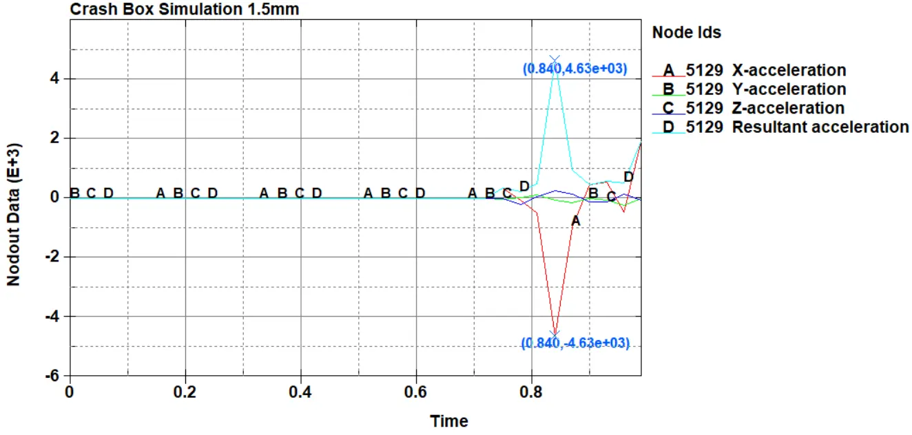
Fig 1.15: Nodal acceleration of a node selected in the middle of the crash box for 1.5mm shell thickness

It is evident from figure 1.13 and 1.14 that nodal acceleration values for 1.2mm shell thickness and 1.5mm shell thickness show identical behaviour. However, the nodal acceleration value for 1.5mm shell thickness is slightly higher (4.63mmms2">4.63mmms24.63mmms2) than 1.2mm shell thickness (4.48mmms2">4.48mmms24.48mmms2). We can see the acceleration values for X direction are negative. This is because the crash box is stopped by a rigid wall and thus deaccelerates. Whereas the resultant acceleration is the magnitude hence positive and almost equal to X-direction acceleration value because Y and Z direction accelerations being very small in comparison.

Energy plots for the crash box:

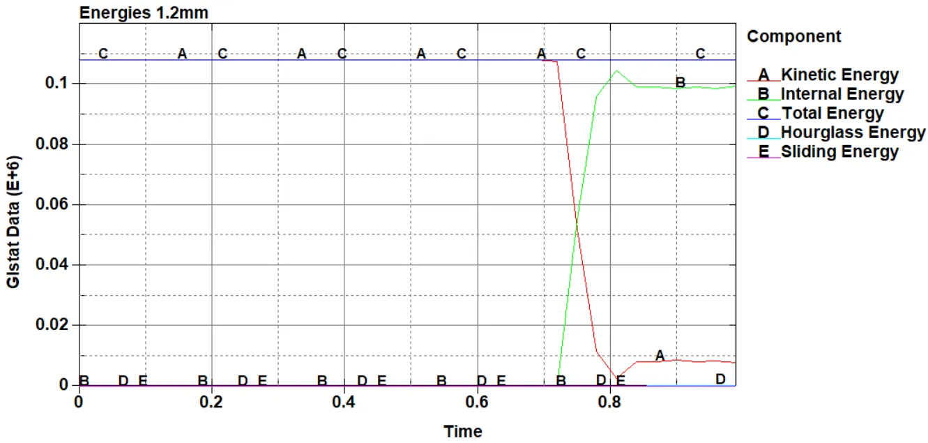
                                Fig 1.16: Energy plots for 1.2mm shell thickness crash box

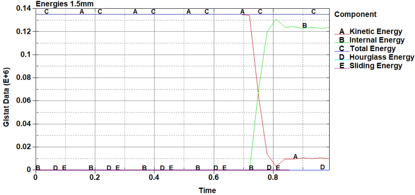
                                     Fig 1.17: Energy plots for 1.5mm shell thickness crash box

From figure 1.16 and 1.17, it is clear that 1.5mm shell thickness crash box possesses higher energies than 1.2mm shell thickness. In both the cases velocity is same but the mass is different. So, the crash box of a higher mass (1.5mm shell thickness) will have higher momentum and energies compared to a lighter crash box (1.2mm shell thickness). The crash box having initial velocity possesses kinetic energy, this kinetic energy is reduced during the impact and converted to internal energy. This can be seen in figure 1.16 and 1.17. The small increase in Kinetic energy and decrease in internal energy after 0.8ms is because the crash box bounces back and gains small velocity. Total energy remains almost constant as there are no other significant energy losses or gains in the system except small plastic deformation. Hourglass energy very small compared to the internal energy and in a desirable range.

Sliding energy is the sum of slave and master energy. But the RCFORC which is ASCII file and calculates contact forces for slave and master does not return anything for single surface contact definition. This is because only the slave side is defined for the single surface contact and master side is undefined. So the forces from only slave sides are present and thus the net force is zero. So the sliding energy for both the cases is zero.

Stress and strain plots for the crash box:

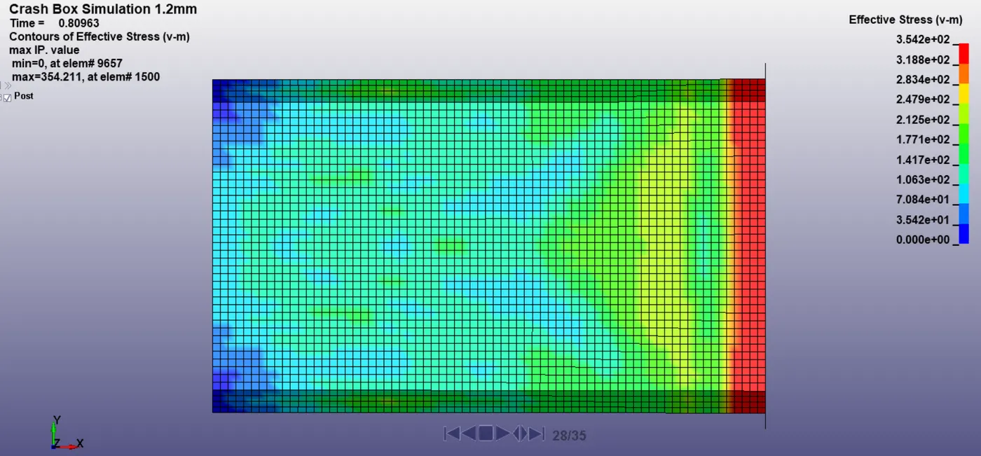
                                Fig 1.18: Effective stress (v-m) for 1.2mm shell thickness

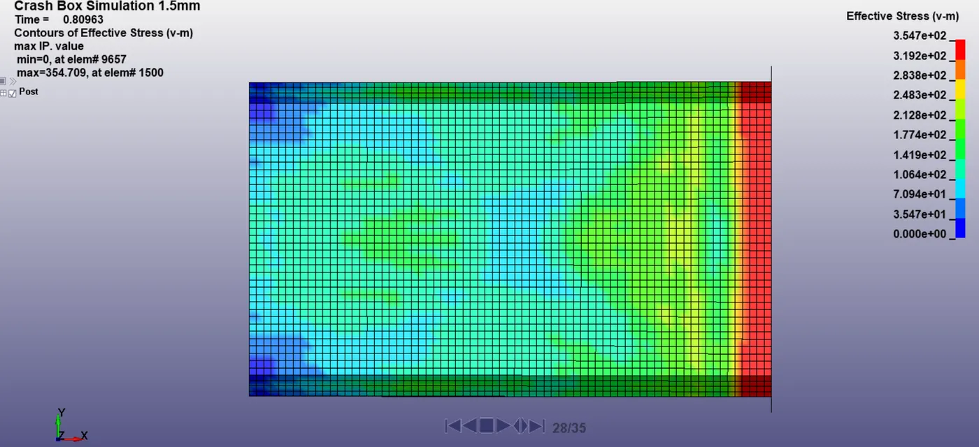
                                Fig 1.19: Effective stress (v-m) for 1.5mm shell thickness

Figure 1.18 and 1.19 shows the effective stress or Von-Mises stress in crash box for 1.2mm and 1.5mm shell thickness. The highest effective stress value for 1.2mm shell thickness is 354.211 MPa and for 1.5mm shell thickness is 354.709MPa. The highest value depicted above is for element number 1500. Figure 1.20 and 1.21 depicts the effective stress behavior for element number 1500 with respect to time for both shell thicknesses. Here we can see the stress value has exceeded the yield stress that is 310MPa in both the cases. This signifies that the material stress has passed the yield point and there is permanent deformation (plastic strain) in the crash box.

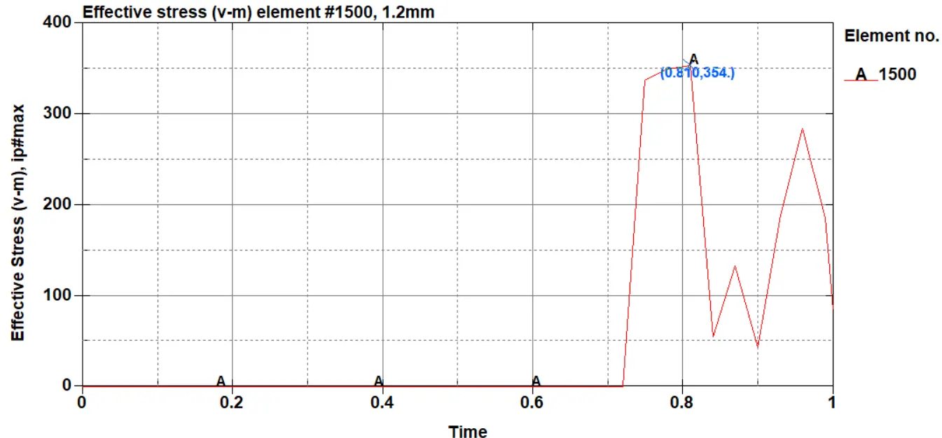
                Fig 1.20: Effective stress (v-m) for element number 1500 and 1.2mm shell thickness

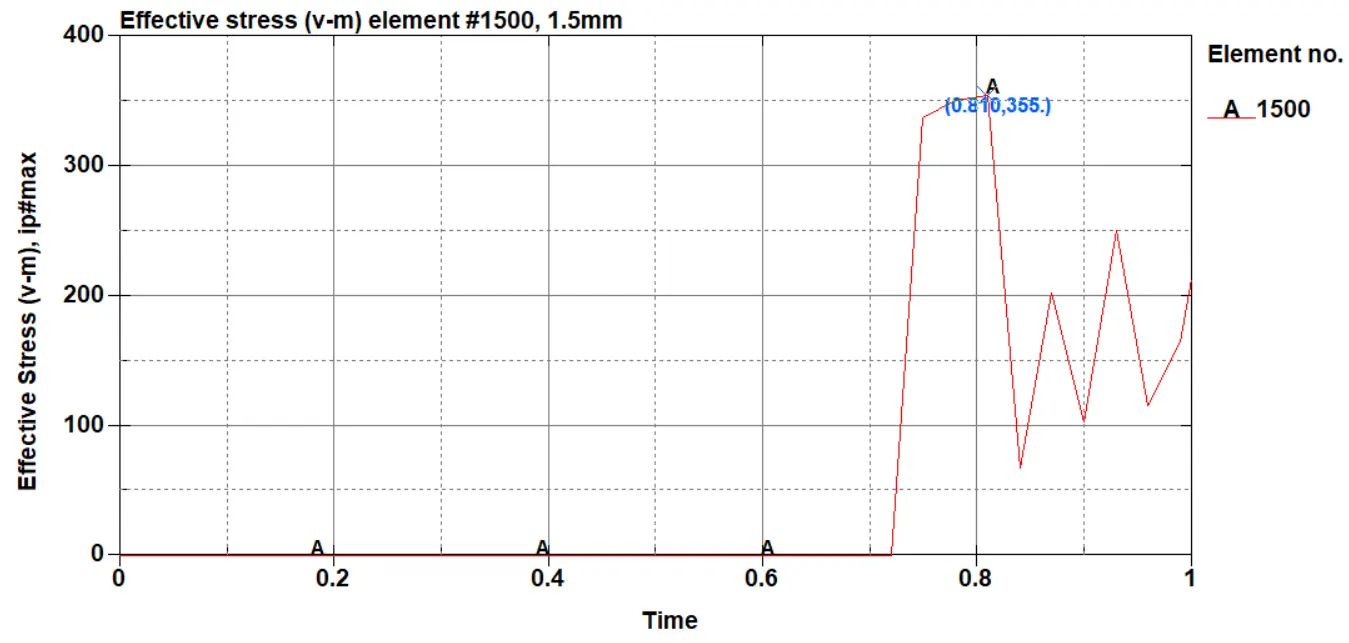
                Fig 1.21: Effective stress (v-m) for element number 1500 and 1.5mm shell thickness

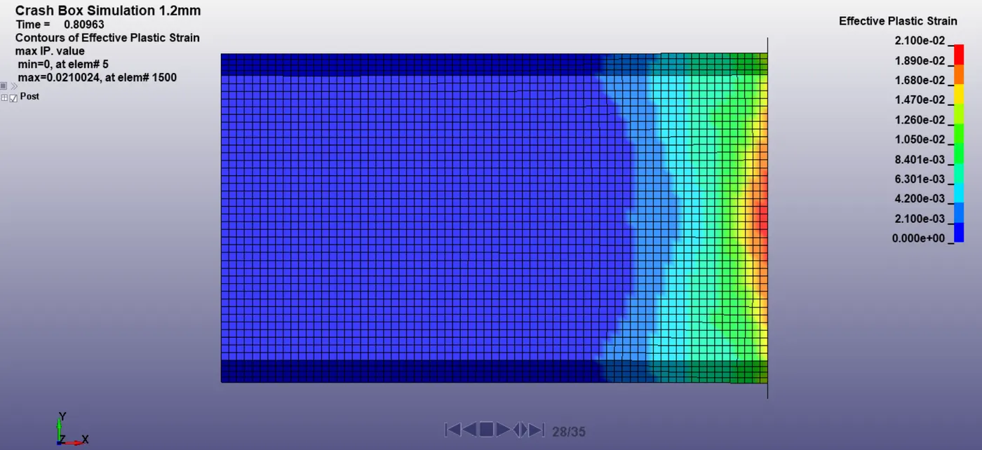
                       Fig 1.22: Effective plastic strain in 1.2mm shell thickness crash box

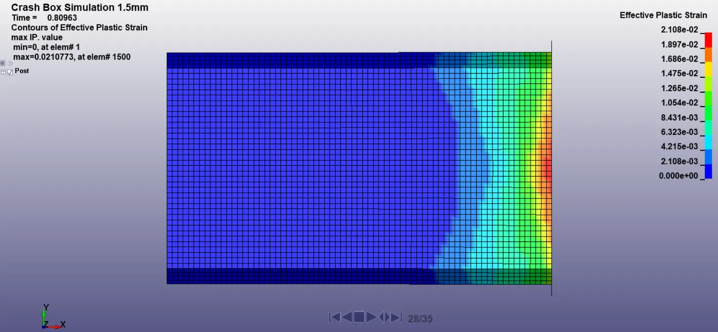
                       Fig 1.23: Effective plastic strain in 1.5mm shell thickness crash box

Figure 1.22 and 1.23 shows the effective plastic strain values on a crash box for both the shell thicknesses. We can see there is permanent deformation (Plastic strain) due to higher stress values than the yield stress. This plastic strain is developed as a result of the impact. Figure 1.24 and 1.25 shows effective strain behaviour with respect to time. The effective plastic strain value of 0.0210024 is seen for 1.2 mm shell thickness whereas 0.0210773 for 1.5mm shell thickness. This deformation is not recoverable and we can see from figure 1.24 and 1.25 this strain value remains constant even after the crash box bounces back.

 

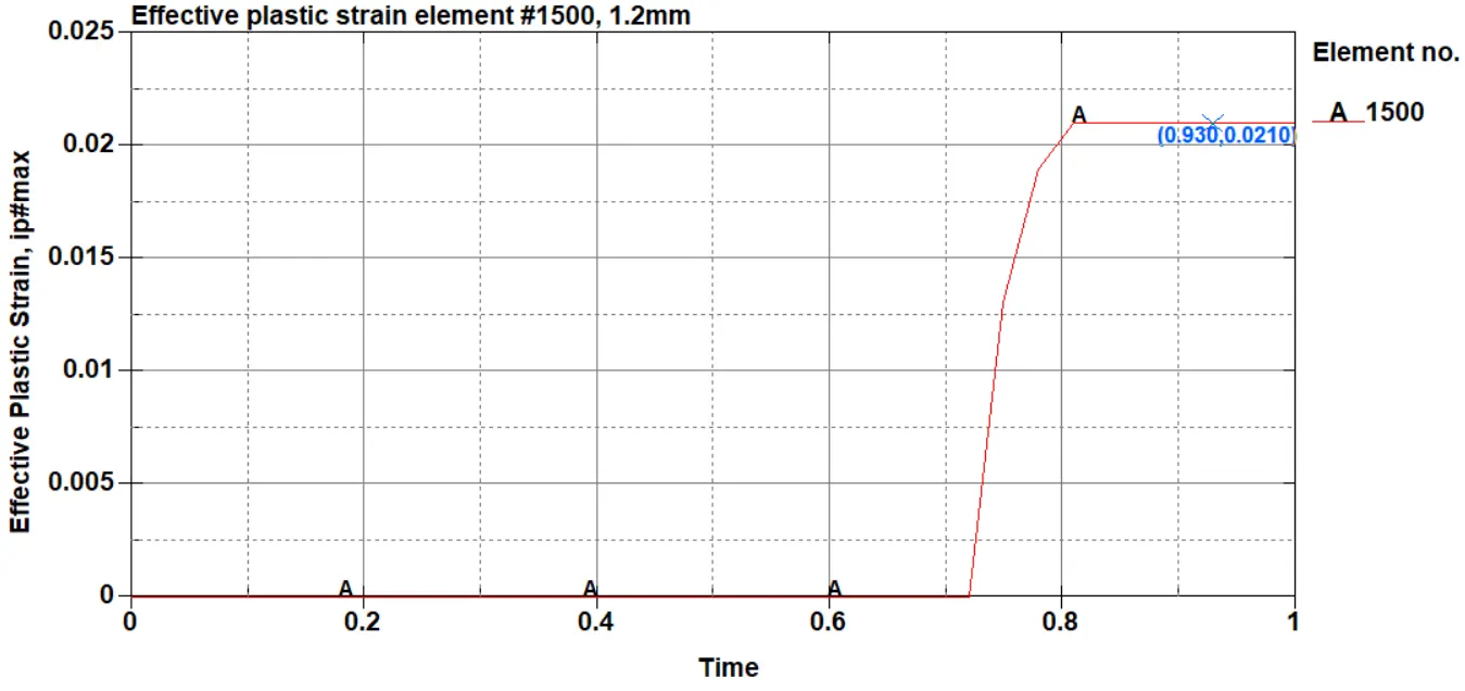
                 Fig 1.24: Effective plastic strain for element number 1500 and 1.2mm shell thickness

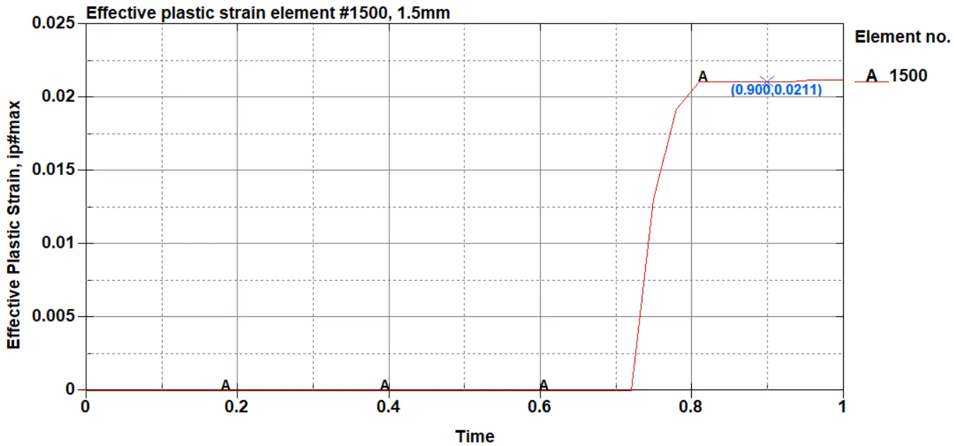
                 Fig 1.24: Effective plastic strain for element number 1500 and 1.5mm shell thickness

CONCLUSION:

The crash box test has been simulated. With considered material properties, the crash box bounces back after the impact.