Week - 4 - Crash Box Simulation

AIM:
To simulate the crash test of the crash box impact on the rigid wall. The given crash box which is meshed has to be setup with 1.2mm thickness and 1.5mm thickness. Nodal accelerations, Directional stress and strain values should be compared.

PROCEDURE:

Crash Box :
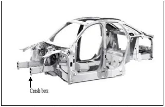
A crash box is a highly energy absorbing structure that crashes on application of loads and reduces impact on other components nearby. The crash box is an important component in determining crashworthiness of a vehicle, and is placed between the bumper and side rails. Automotive manufacturers aim to reduce vehicle weight in order to meet economic and environmental concerns without sacrificing on safety standards for car crashes set under the Federal Motor Vehicle Safety Standards.



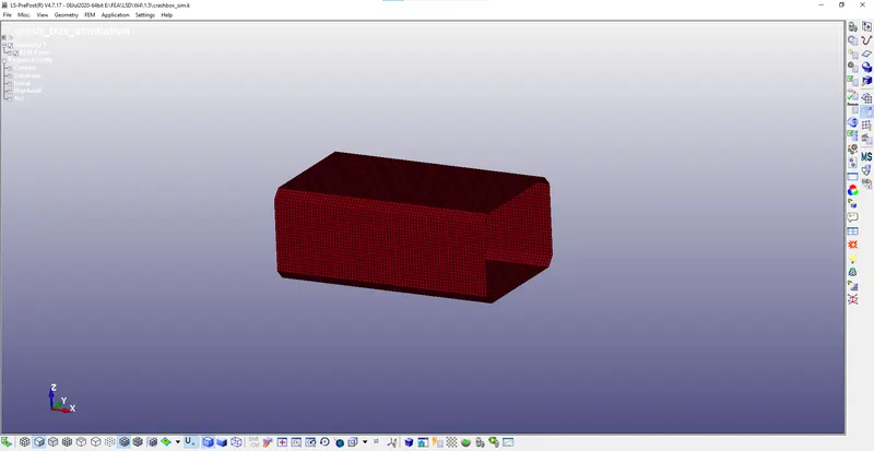
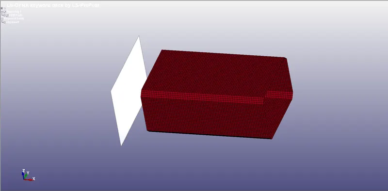
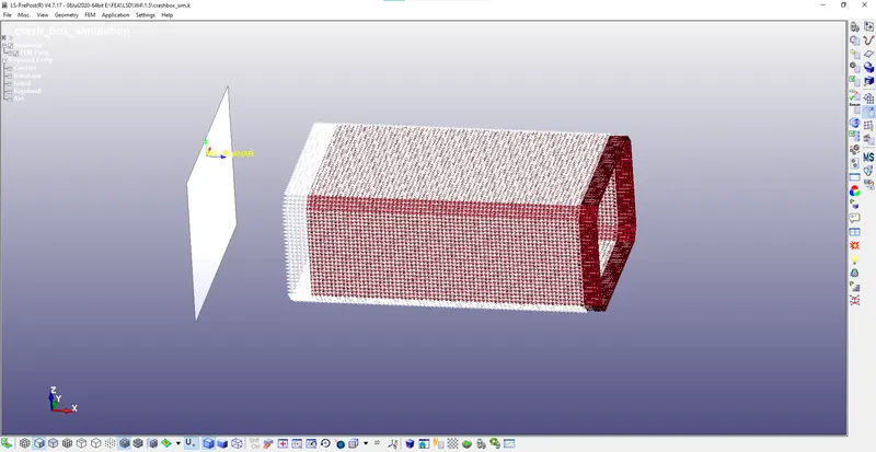
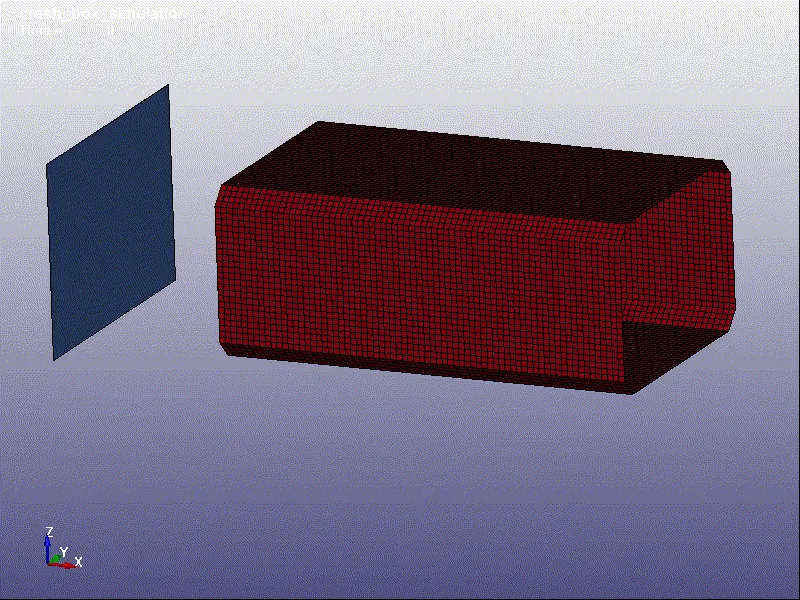
1. The given crash box model is a meshed model with just the basic keywords set in it. It is a single part with shell elements. Here is the given parent model :



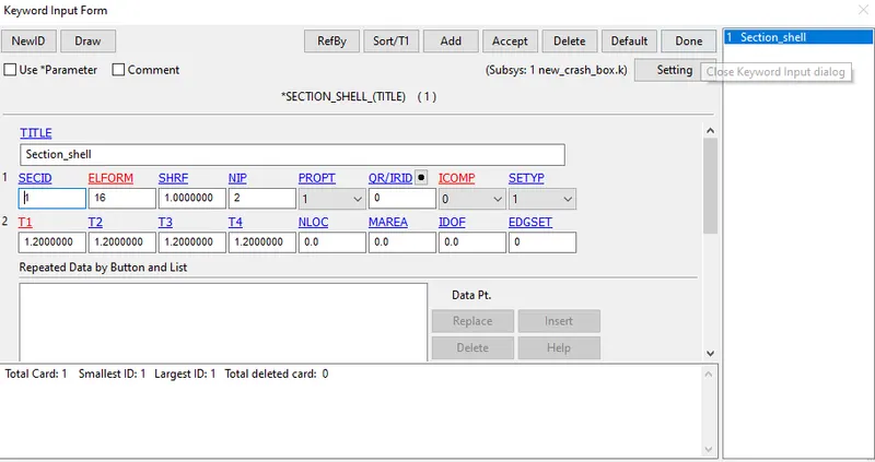
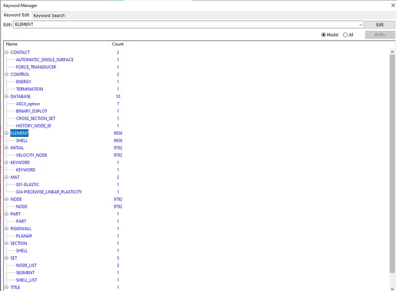
2. Now, we should first create a shell section for the crash box. To create the shell section, go to Model & part >> Keyword Manager >> Section >> Shell. Provide the Section ID, Provide the other entities ELFORM as 16 ( for fully integrated elements ) since the model is not so complex. Then provide the thickness T as 1.2mm (This has to be changed to 1.5mm & the same simulation has to run to compare the study on both the models)



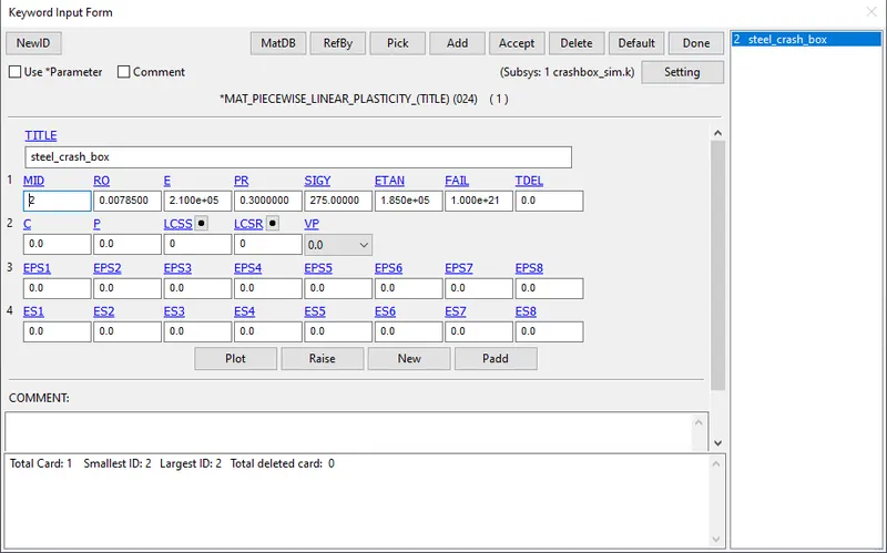
3. Now, once the section is created, we need to create the material for the part. Here we are using the MAT_024 Piecewise Linear Plasticity with the properties of the steel. Initially, the simulation can be run with the Elastic material card MAT_001 to check whether the simulation setup is running correctly. Then we can change the Material card to MAT_024. The appropriate Steel properties were entered. The Carbon Steel S275 grade properties are entered with the Tangent modulus defined. The Tangent modulus defines the Stiffness of the material beyond the Elastic limit in the Plastic region. Usually the Tangent Modulus would be around 16% of the Young's modulus of the corresponding material.



4. Once the Material and the Section is created, Now we can Update them in the Part such that they are assigned to the crash box respectively. After Assigning the Material and the Section, Now we create the Rigid wall for the crash box to Impact. The Rigid wall is created by Create Entity >> Rigidwall >> Planar >> Select a node >> Translate the Plane to certain distance in -x axis. Thus, the Rigid wall would be created.
In the Keyword Manager, Go to Rigidwall >> Planar >> Create the Slave node set by including all the nodes in the crash box as slave to the Rigid wall.




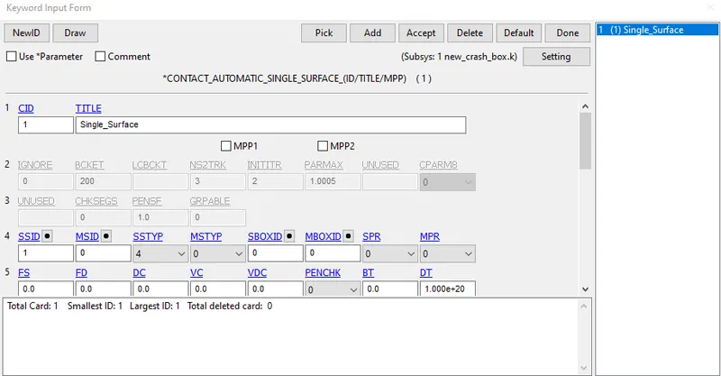
5. Once the Rigidwall is created, Now we should create the Contact Interface for the parts. Here what we expect is when the crash box is impacting on the rigidwall, mostly there are chances for the crash box to buckle. In general, all the crash cases, even in the event of car crash simulation, the object under study is always given a self Impact interface. In order to create the self Impact interface, go to Keyword Manager >> Contact >> Automatic single surface >> SSID >> Select the Slave Set as the whole Crash box. We don't need to define the Master set here since the slave is the master in this case.



6. Now, we need to create certain parameters to accquire the results from the Impact simulation. We need to compare the directional stresses, acceleration of the particular node, cross sectional forces in the crash box.
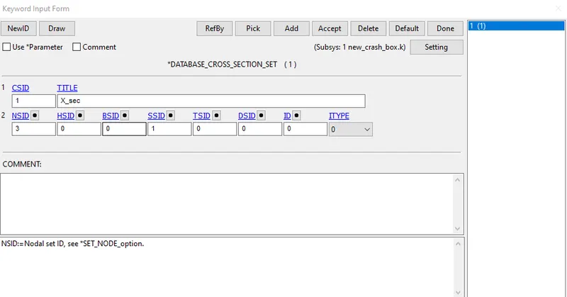
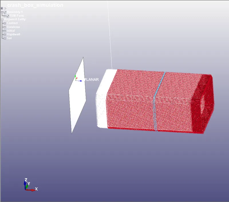
Firstly, to study the cross sectional forces, we need to create a cross section so as their results can be studied. Go to Create Entity >> Segment >> Shell >> Select the respective elements. Similarly, create a Set_node >> select the nodes that define the cross section. Now, we need to define them in the Database.
So, go to Keyword manager >> database >> Cross section Set >> Select the Set of elements >> Provide Cross section ID and accept and done.





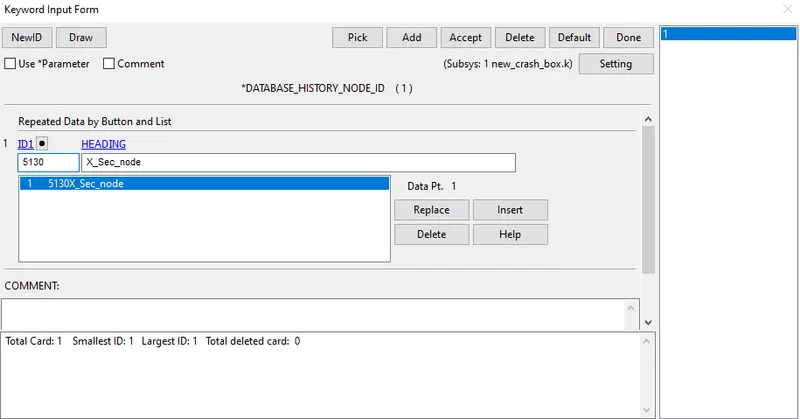
7. Now, we need to study the acceleration on the specific node in the crash box. To study them, we need to create *History_NodeID and NODOUT in the Database and the ASCII option. Go to Keyword Manager >> Database >> History_nodeID >> Pick the Node and Select the ID >> Provide ID for it >> Accept and Done. Now, to get the output of that node, define the NODOUT file in the ASCII option while requesting the output.




8. Now, we need to Provide the Initial velocity for the model. Here, we have two options, Either we can create a moving rigidwall and constrained Crash box or else we can simply apply the velocity on the crash box. The velocity to be applied is around 50Kmph which is around 13.89mm/ms. It has to be applied to the whole crash box in the -X axis to make the crash box hit the rigid wall. Go to Create Entity >> Inital >> Velocity >> Vx >> -13.89 >> Select the whole crash box part as the entity and accept and done.




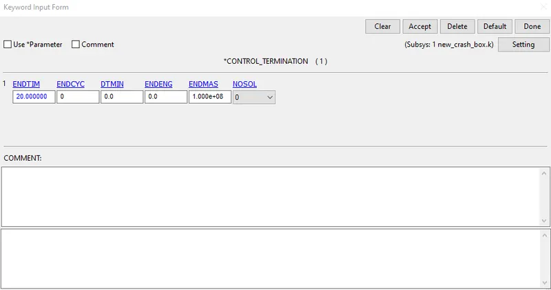
9. Now, we need to set the termination time for which the crash simulation has to carry on. Go to Keyword Manager >> Control >> termination >> 20ms >> accept & done.



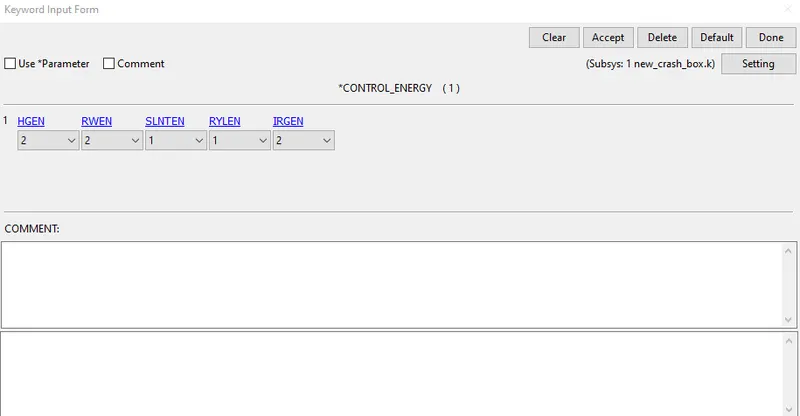
10. Similarly, create control card for the Hourglass energy. Keyword Manager >> Control >> Hourglass >> HGEN >> 2 and all the other properties were set to control the Hourglass energy. Since we use fully integrated elements, the presence of Hourglass energy is less likely to happen.





11. Thus, all the required entities were created, we can now define all the output requests. For the output requests, go to Keyword manager >> Database >> D3Plot >> enter DT >> 0.1 >> accept & done. Then, Cross_section_set and History_nodeID were already been created.
Now, ASCII options were to be selected. Keyword manager >> ASCII >> GLSTAT, MATSUM, RCFORC, NODOUT, SECFORC, NCFORC, SLEOUT. For all these files, Enter corresponding DT as 0.1 >> accept & done.
After all the entities were created, we can use Keyword check to see If there are any errors in the keywords defined. If the errors are not present, we can save the Keyword and can run the file in the LS-Run.




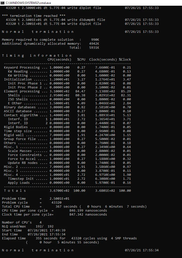
Now, Open the LS-Run, Open the saved .K file and run the simulation. See whether the simulation ends with normal termination.




Let's see the results. To open the animation file, Open LS-Prepost and File >> Open Binary File >> D3PLOT file.



Let's open the GLSTAT plot to see the global variables like Internal energy, Kinetic energy and total energy of the crash box simulation. Load the *glstat file and then Select the required global variables and click on Plot.

Global variables Plot :



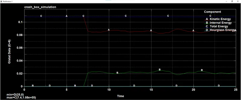
Here as the plot implies, the Hourglass energy is almost non existent as we use fully integrated elements. Also, the Kinectic energy decreases when the crash box impacts on the rigidwall and at the same time the Internal energy Increases. The total energy of the system thus remained constant throughout and the value was about 0.12E+06 gm.`frac(mm^2) (ms^2)`

Now, Let's see the Cross sectional forces developed in the crash box during the Impact. To open them, Go to ASCII >> SECFORC >> Load >> Select the Cross section ID >> Resultant Force >> Plot.

Cross sectional force :



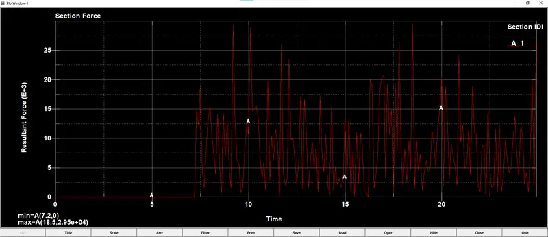
As we can see that the cross sectional forces varies once the Impact happens, however there are several ups and downs in the plot which is because the crash box rebounces once the impact happens which causes them to have some energy in it. This fluctuation is due to the fact that the crash box rebounces and carries away those Impact energy within it. The maximum value reached was about 2.95E+04 N.

Now, Let's see the Nodal acceleration on the crash box which has 1.2mm thickness value with the properties of Steel. To see them, ASCII >> NODOUT >> Select the NodeID >> Resultant Acceleration >> Plot.

Nodal acceleration on 1.2mm Thick Crash box :



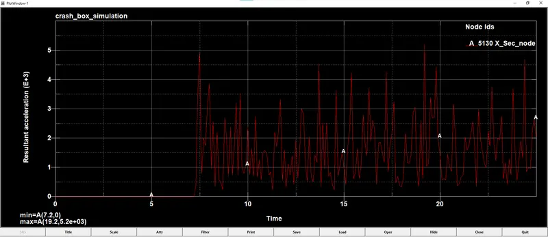
As we can see that the maximum acceleration reached by the node in this Impact is about 5.2`frac (mm) (ms^2)`

Let's check the Nodal acceleration of the crash box with 1.5mm thickness value.

Nodal acceleration on 1.5mm Thick crash box :



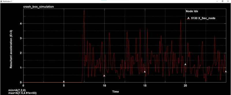
In this case the maximum nodal acceleration attained was about 4.91 `frac (mm) (ms^2)`

Now, Let's compare the Directional stress and strain values of both the cases.

X & Y stress values of 1.2mm thick crash box :

X-Stress on 1.2mm thickness :



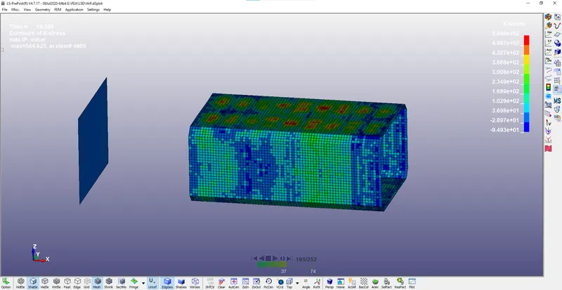
From the above simulation, we can see that the maximum value reached was about 564.6 Mpa. This was happened around 19.399ms of the run time which we've provided.

Y-stress on 1.2mm thickness :



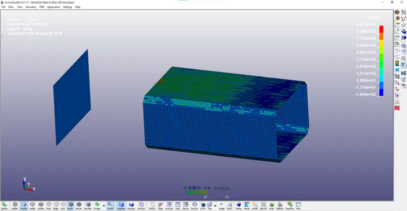
The maximum stress value along the Y-direction was found to be 937.1Mpa.

Now, Let's check the values of strain in the same 1.2mm thickness crash box,

Effective Plastic strain on 1.2mm thick crash box :



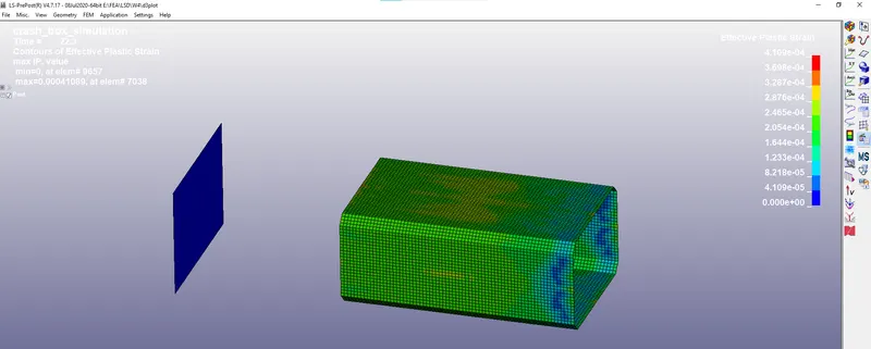
The Maximum Plastic strain in the 1.2mm thick crash box was about 0.00041.

Directional stress on 1.5mm thick crash box :

X-stress on 1.5mm thick crash box:

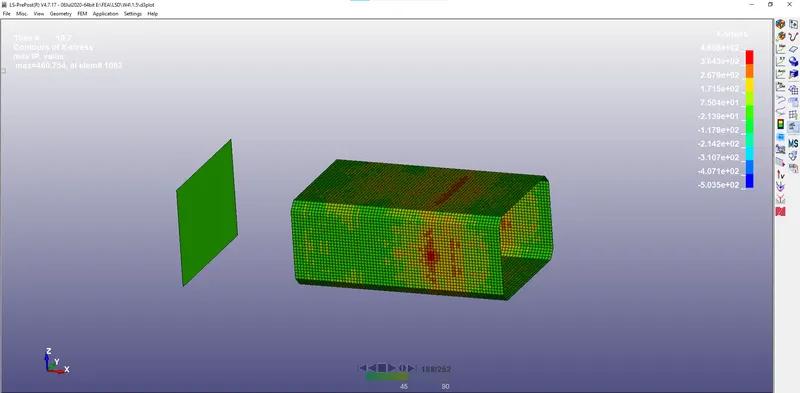
The maximum stress value created was about 460.75Mpa. This value is comparitively less than the crash box of 1.2mm thickness. Now let's see the values obtained along Y-axis stress.

Y-stress on 1.5mm thick crash box:



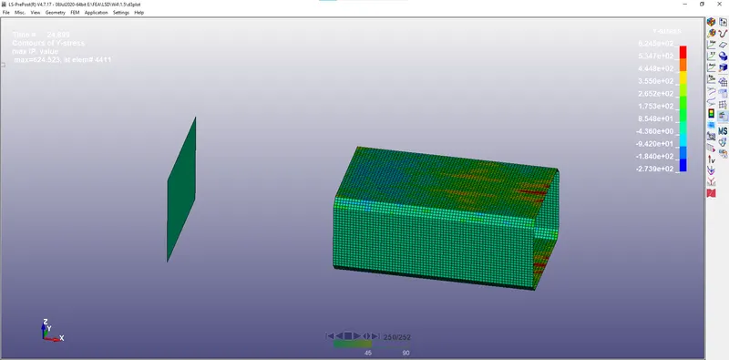
The maximum stress value along Y-axis is around 624.5Mpa which is also quite less than the crash box of 1.2mm thickness.

Effective Plastic strain on 1.5mm thickness crash box:



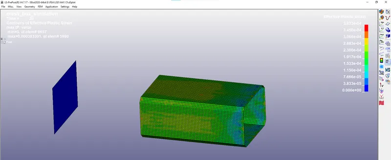
The strain effects were not so evident in both the cases. However it is still less in 1.5mm thick crash box with 0.00038 than the one with 1.2mm thickness.


Comparing various attributes of crash box with 1.2mm thickness and 1.5mm thickness :

S.no	Description	Value on 1.2mm	Value on 1.5mm
1.	Nodal acceleration	5.2 `frac (mm) (ms^2)`	4.91 `frac (mm) (ms^2)`
2.	X-Stress	564.6 Mpa	460.75 Mpa
3.	Y-Stress	937.1 Mpa	624.5 Mpa
4.	Effective Plastic Strain	0.00041	0.00038

Thus, the crash box Impact simulation is carried on both thickness values 1.2mm and 1.5mm and their results along various entities have been studied.


RESULTS :

Here, we can see that the values obtained in 1.5mm thick crash box is comparitively higher than the crash box with 1.2mm thick crash box. Since there is no role for geometric stiffness change, the dimensional stiffness plays a vital role here. Thus, If there is no limit in terms of weight factor, we can use 1.5mm thickness crash box which provides better values. Thus, the comparison of crash tube of various thickness and its simulation is done successfully.