Week 4 - CHT Analysis on Exhaust port

Conjugate Heat Transfer analysis on Exhaust Port

Aim : To simulate the flow of hot exhaust gases through an exhaust port and see how the heat transfer takes place and verify the same.

Introduction:

Conjugate heat transfer co efficient refers to accurately predicting heat transfer between the fluid and the body by simultaneous solving all the relevant solid and flow field heat transfer processes. In CHT, wall heat transfer coefficients and their local variations on surfaces are directly calculated within the model rather than based on simplified empirical calculations. The CHT approach therefore has benefits for those applications where heat transfer is either non-uniform or difficult to calculate empirically.

The CHT analysis plays a major role in designing the heat exchangers such as coolers, heaters and in the field of air conditioners, electronic products cooling, radiators and many more. Here we are trying to analyse the heat transfer in a 4 cylinder inline engine between the hot exhaust gases and the wall of exhaust manifold.

Geometry preparation

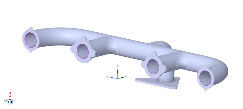
The CAD model of the exhaust port is loaded on to the space claim and the solid volume (exhaust port) inside which the gases flow and this solid volume acts as an enclosure to the gas flow is as shown below.

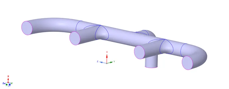
The next step would be to extract fluid volume out of the soild volume using volume extract feature. This is the volume in which the exhaust gases flow

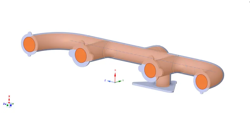
The image below shows both the solid and fluid volume together. We can see 4 ports through which the exhasut gases enters at high temperature and has a single outlet to which all the inlet port connects. Since the fluid is flowing inside a pipe(exhaust port) there is no need for creating an enclosure. We have to make sure that the mesh of the outer surface of Fluid volume and inner surface of solid volume are connected and continuous using the share topology option. This is done in order to initiate the heat transfer between the fluid and the exhaust manifold wall.

Meshing

Balancing accurate results to the processing power and time required is an important aspect of CFD, hence a comparison to a simple baseline mesh and a much refined mesh is done.

Case 1 : Baseline mesh

• Element size : 0.15m
• Number of elements : 137298
• Number of nodes : 27380

Case 2 : Refined mesh

• Element size : 0.075
• Number of elements : 1124123
• Number of nodes : 397835

Baseline mesh

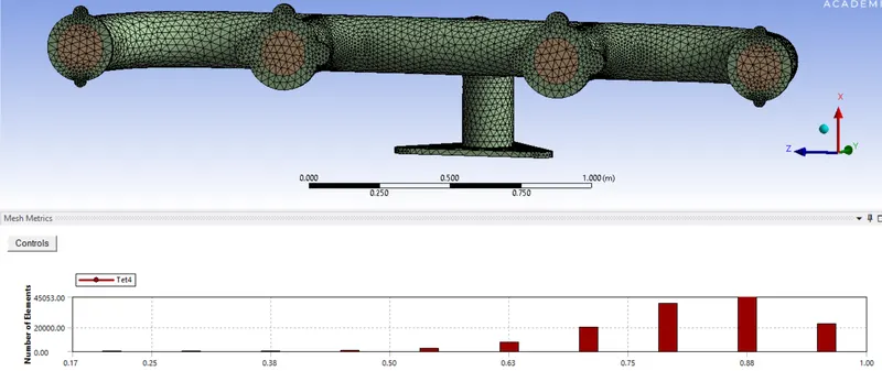
The image below shows the simple mesh. This is the step where the parts of the prepared geometry is named, i.e, Inlet ports, outlet port and the outer wall. The element size defined here is 0.15m which is default size and is enough for baseline mesh.

We can also see the mesh quality in the image below and it can be observed that the least quality is somewhere between 0.17 and 0.25 which is better than 10% hence it can be inferred as a good enough mesh.

The image below shows that the mesh of the fluid volume corresponds and is continous with the mesh of the solid volume.

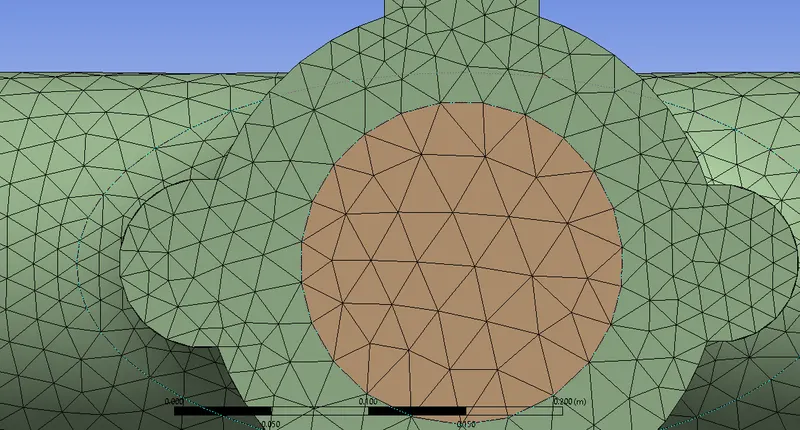
The mesh of the solid Volume of the exhasut manifold can be seen in the image below.

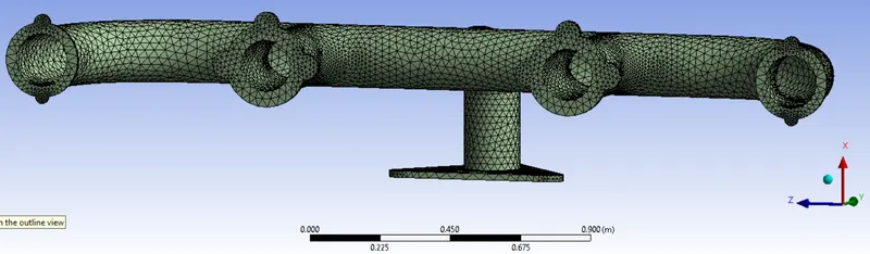
The meshing of the Fluid volume inside the exhaust manifold can be seen in the image below.

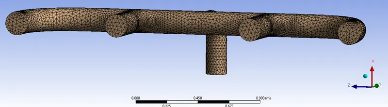
Refined mesh

Refinement of the mesh can be done in many ways. Here we decrease the element size of the mesh from 0.15m to 0.075m. The quallity of the mesh can also be seen in the image below where the least is in between 0.11 and 0.25.

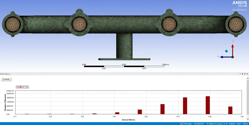
The image below shows refined mesh of solid volume

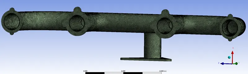
The image below shows refined mesh of fluid volume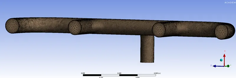

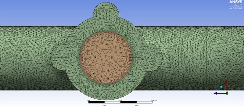
Body sizing method is applied to the exhaust manifold in order to further refine the mesh and to obtain an even boundary layer to get the heat transfer between the fluid and the inner wall of the exhaust manifold which is in direct contact with the gas flow.

Y+

After the simulations, the Y+ of the baseline mesh was found to be 448.90 which does not make sense, but the Y+ in the refined mesh is supposed to be above 30 and in order to be on the safer side, a Y+ of >60 and <500 is considered for the turbulance model under the logarithmic law and after the simulation it was found to be 441.60

Pre-processer set up

Solver setup

• Set up type - Pressure based solver
• Time - Steady state simulation
• Absolute velocity formulation
• Viscous model - K-epsilon (2 equation)
• Fluid material - air
• Solid material - Alumunum (al)
• Inlet velocity - 5 m/s
• Inlet temperature - 700K
• Air Density - 1.225 `(Kg)/ (m^3)`
• Soild density - 2719 `(Kg)/ (m^3)`

Results

Baseline mesh :

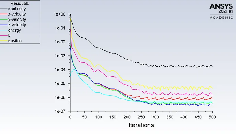
The image below shows the plot of change of Residuals with respect to iterations and we can see that somewhere between 250 and 300 iterations the system has reached steady state.

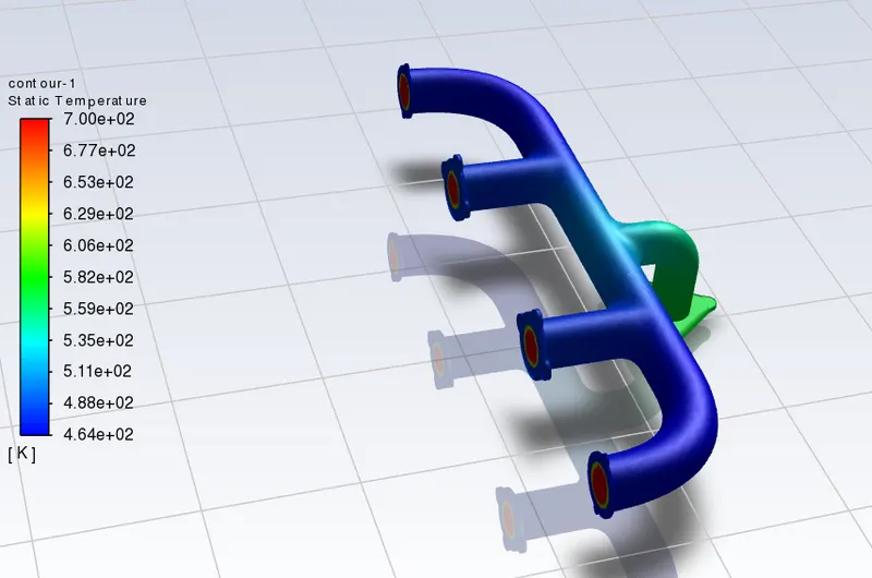
In the image below we can see the final distribution of the Static temperature on the walls of exhaust manifold. As we can observe that the temperatue is higher near the single exhaust outlet compared to 4 exhaust inlet. Since the pressure, velocity and exhaust gas density is higher at the outlet side, the contour is as expected.

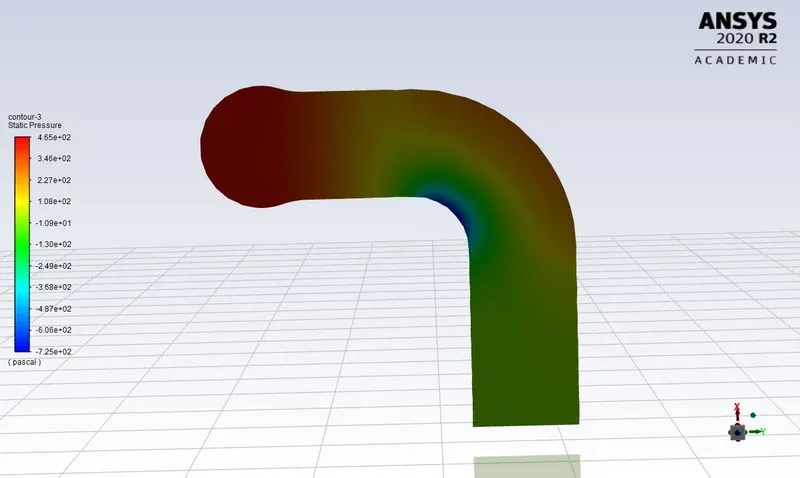
The image below shows pressure contour on cut section plane and as we know low pressure created region means that the air speed is higher and at the bend of the throat the inner wall has lowest pressure, hence the velocity expected to be highest there.

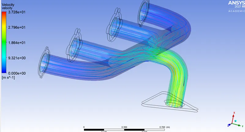
Velocity streamlines of the exhaust gases can be seen in the image below. The gases from 4 inlets are converging into one outlet which has lead to the increase of velocity at the junction and is highest at the lower part of the outlet pipe bend which means that the surface heat transfer will be highest at that point.

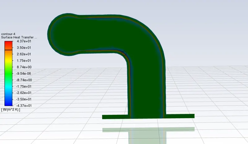
The cut XY plane shows surface Heat transfer co efficient at the inner walls of the exhaust port and as expected from the velocity streamline plot we can see that the highest heat transfer takes place at the throat bend.

Refined mesh :

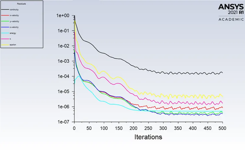
The image below shows the graph of residuals and can be observed that after 200 iterations the simulation has reached its convergence.

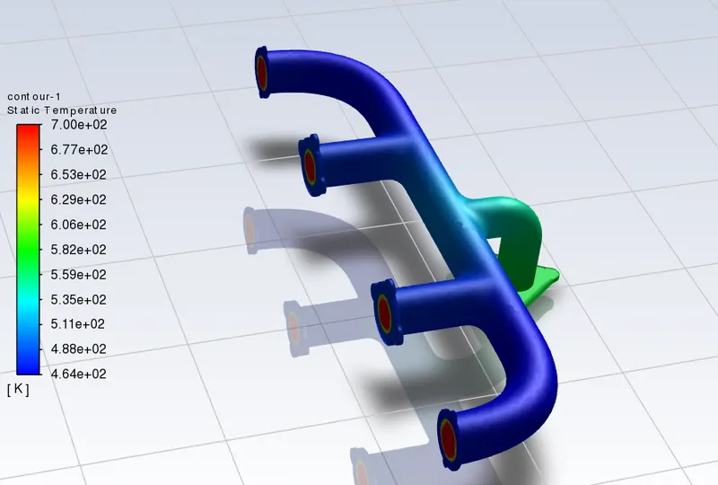
The image below shows the Static temperature contour over the exhaust manifold. As we can see that the temperature is high at the pont of intersection of all the ports and gets higher as we go down towards the outlet port.

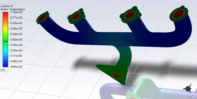
Here we can see the bottom part of the exhaust manifold and we can observe the significant higher temperatures near the outlet compaerd to inlet.

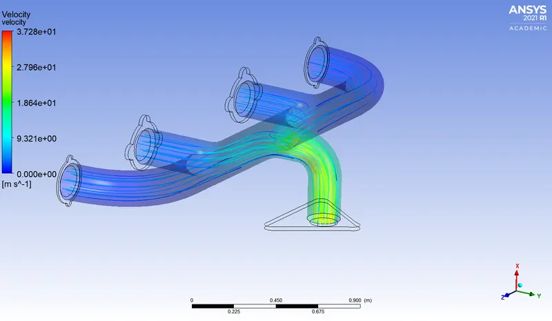
In the images below we can see the Velocity streamlines of the exhaust gases flowing through the manifold and we can observe that at the point of intersection of all inlet ports, the density of the velocity streamlines is high and also the speed increases due to high pressure at the junction. As the velocity increases, so does the flow turbulance and more the turbulant flow, more will the heat transfer.

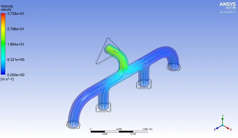
Since we can see higher density of velocity stramlines and with higher velocity at the bottom of the flow cross-section, we can expect the heat transfe to the walls of the manifold to be higher at this point.

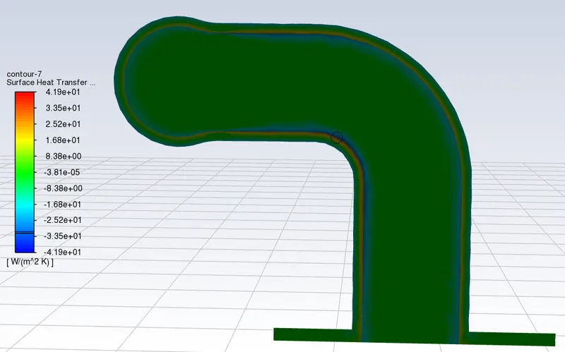
The image below shows the surfeace Heat transfer coefficient on the XY-plane cross section. Since we expected the heat transfer to be highest at the lower wall, it can be confirmed from this view as we can see thicker reddish band at the lower wall bend compared to other areas.

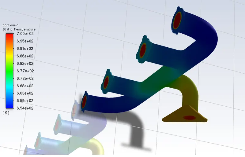
In realistic situation the exhaust gases will have higher velocity. A refined mesh simulation was carried out to see the differences. Due to the higher velocity the heat transfer was more and the temperatue distribution contour cam out as seen in the image below. As we cna observe the outlet end temperature of the exhaust manifold is far higher than compared to one with 5m/s. The velocity considered for this case is 125m/s.

Factors affecting the accuracy

After the simulation of the exhaust port with a baseline mesh and refined mesh, we can conclude that the foollowing factors can be considered in improving the result accuracy

• Mesh sizing and refinement
• Using correct viscous model
• Running the simulation long enough for it reach steady state
• Maintaining y+ above 31 and below 500 for the turbulance model
• Using correct boundary condition values

Conclusion

The simulation of the exhaust gases through the exhaust manifold to check the temperature distribution and heat transfer to the solid exhaust port, following results were obtained:

Type of Mesh	Number of elements	Number of nodes	Surface Heat transfer Co. efficient `(W)/(m^2 K)`	Wall Heat transfer Co. efficient `(W)/(m^2 K)`	Velocity
Baseline mesh	137298	27380	43.692	100.733	5m/s
Refined mesh	1124123	397835	44.914	100.3453	5m/s
Refined mesh	1124123	397835	36.033	1478.854	125m/s

• From the images of the results, it can be inferred that the refined mesh simulations generated smoother gradient and much better contours in the plots.
• The heat transfer co-efficient for aluminum (exhaust material) when the air velocity is 3m/s is between 59-64 `W/(m^2 K)` according to a research and the trend from 1m/s to 3 m/s showed increasing heat transfer coefficient values.
• As we can see the results of wall function heat transfer coefficient we obtained from the simulation for baseline mesh and refined mesh are not varied a lot and are almost equal.