Mixing efficiency
AIM
The main aim of this CFD simulation is to determine the factors affecting the mixing efficiency of 2 fluids at different temperatures through a tee section using ANSYS Fluent and comparing the results
MODEL
The image below shows the model of the tee through which of which the mixing efficiency is simulated. The cold fluid is sent through the top i.e. along the y axis, while the hot fluid is flowing through the tee along the x axis. 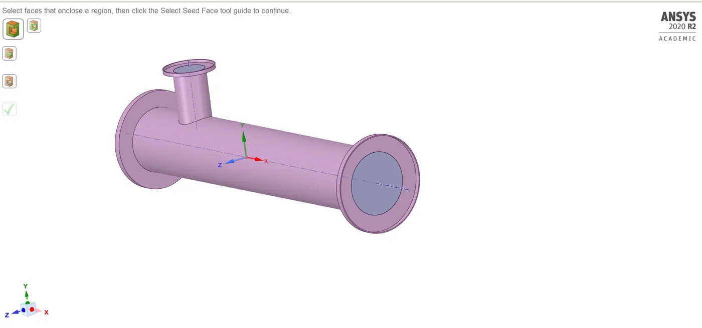
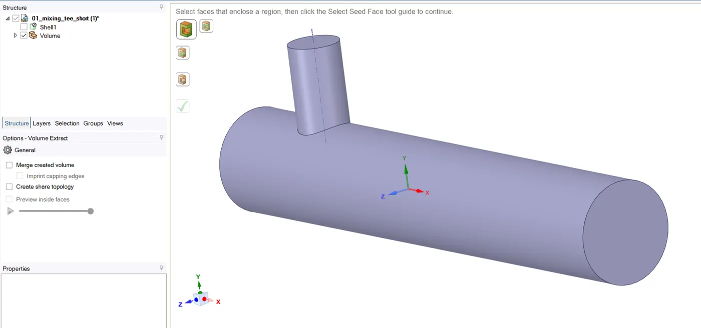
The image below shows the part of the model that is selected to simulate the flow of the working fluid and this is boundary in which the fluid interactions take place.
MESHING
Image below shows the fine meshing of the mixing tee.
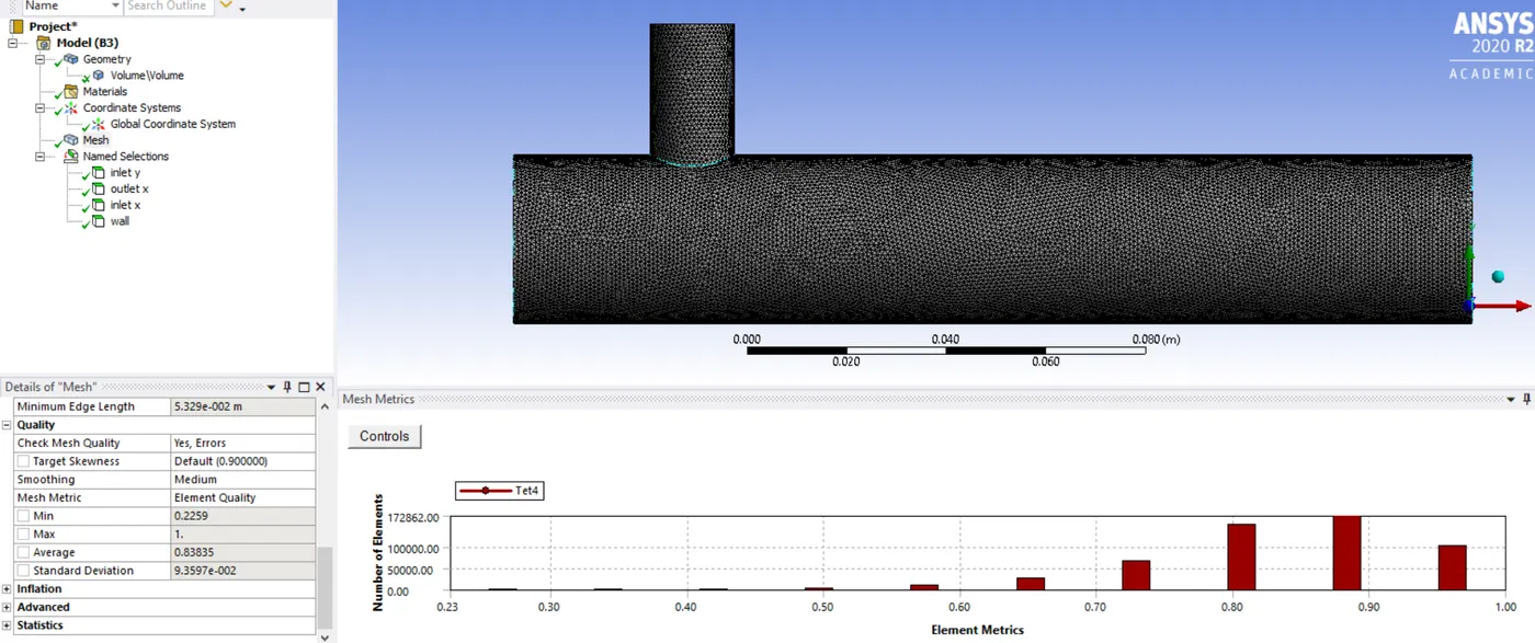
Image below shows the coarse meshing of the mixing tee.
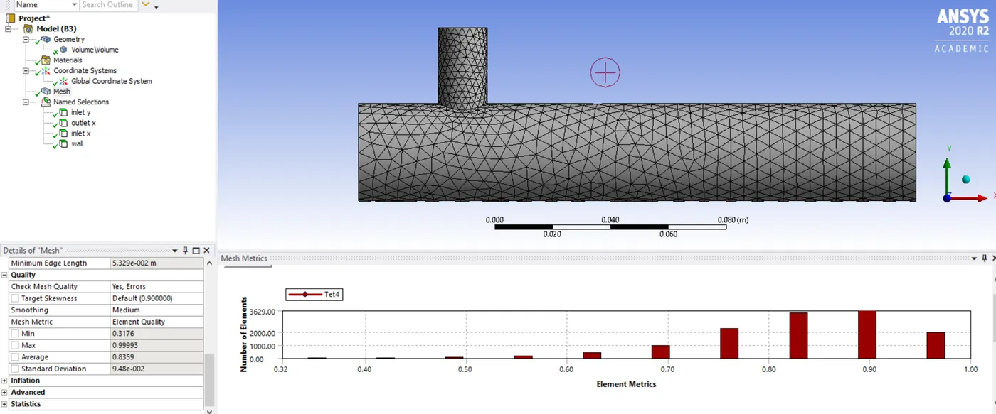
From the above images we can see that the quality of coarse mesh is spread out less and is better compared to fine mesh. The time taken to solve the coarse mesh is less and the results doesn't deviate much compared to fine mesh, hence for this simulation we will be usind the coarse mesh.
SETUP
The following are the given physical conditions :
The pressure conditions outside the mixing tee is atmospheric.
Cold inlet temperature = 19C
Hot inlet temperature = 36C
Case 1: short mixing tee
hot inlet velocity : 3m/s
Momentum ratio = cold inlet velocity / hot inlet velocity
For momentum ratio = 2
cold inlet velocity = 6m/s
For momentum ratio = 4
cold inlet velocity = 12m/s
Case 2: long mixing tee
hot inlet velocity : 3m/s
Momentum ratio = cold inlet velocity / hot inlet velocity
For momentum ratio = 2
cold inlet velocity = 6m/s
For momentum ratio = 4
cold inlet velocity = 12m/s
Solving
For solving the problem, we use K-epsilon model available in ANSYS Fluent. The interaction surfaces are named according to their functions such as :
inlet x
inlet y
outlet x
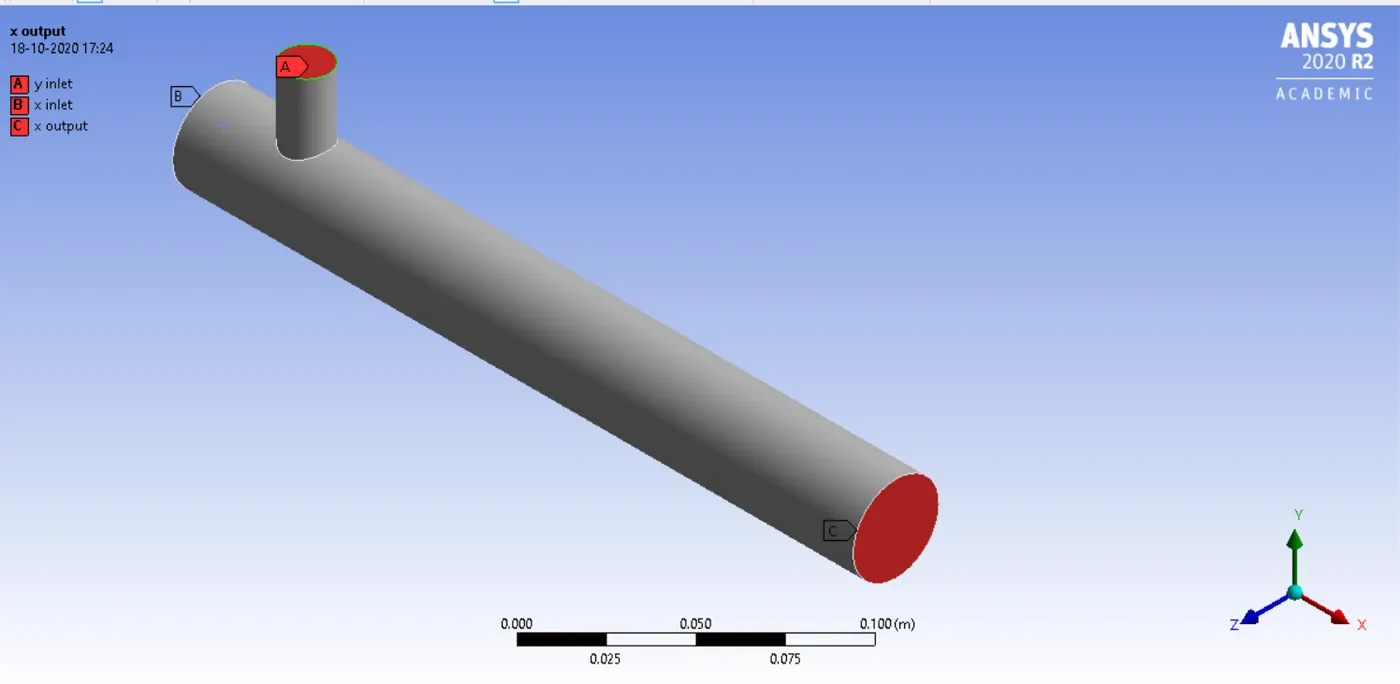
During solving phase the boundary conditions are provided as per the case conditions. These cases are then iterated to convegre to a solution.
Results
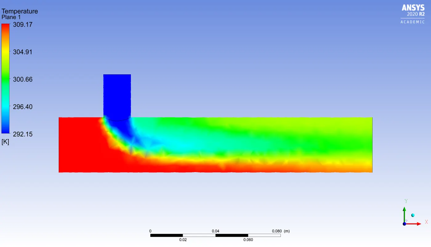
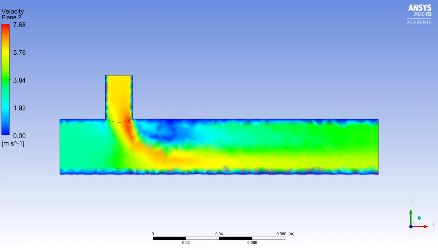
Short mixing tee for momentum ratio 2
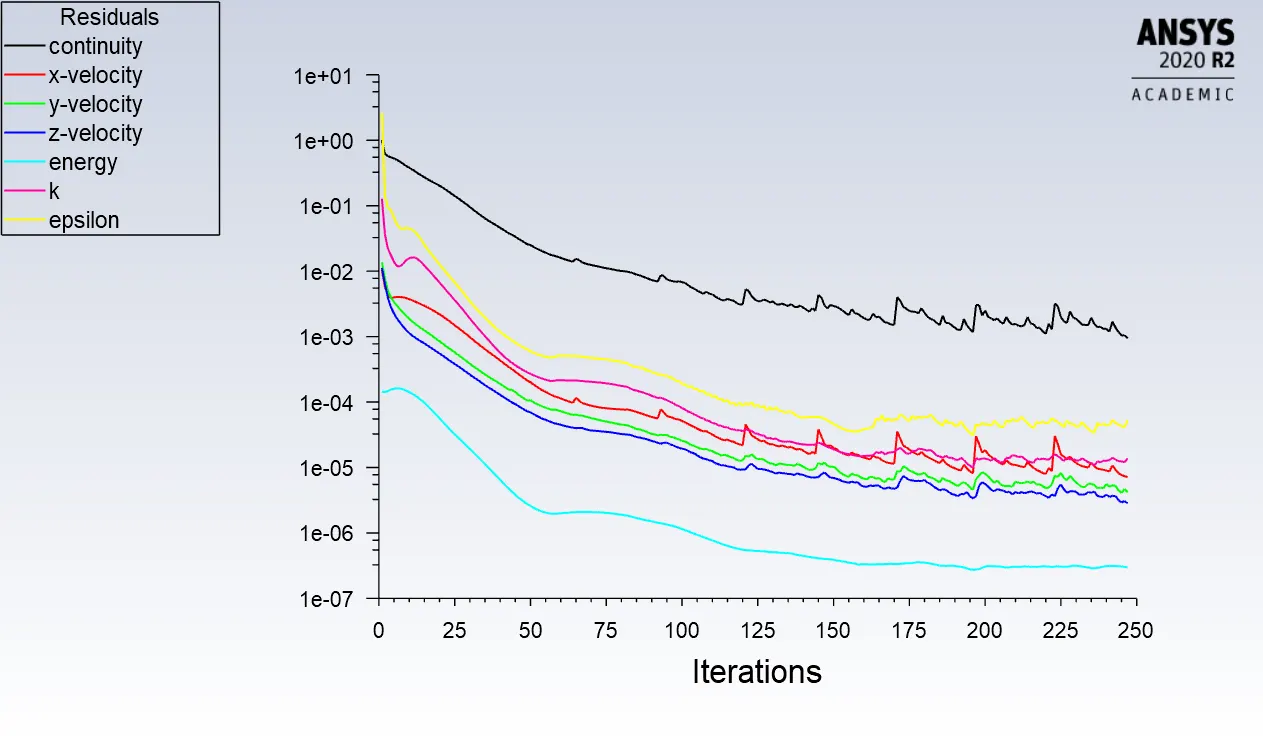
Residuals plot:
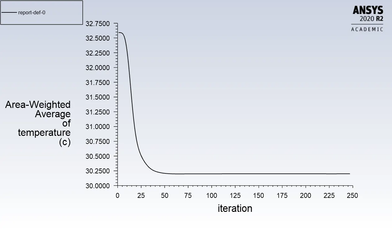
Plot showing Area weighted average of temperature to number of iterations:
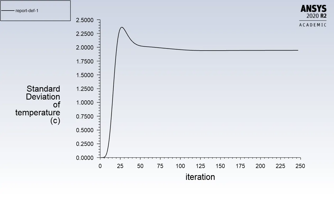
Plot showing Standard deviation of temperature to number of iterations:
Temperature contour plot
Velocity contour plot
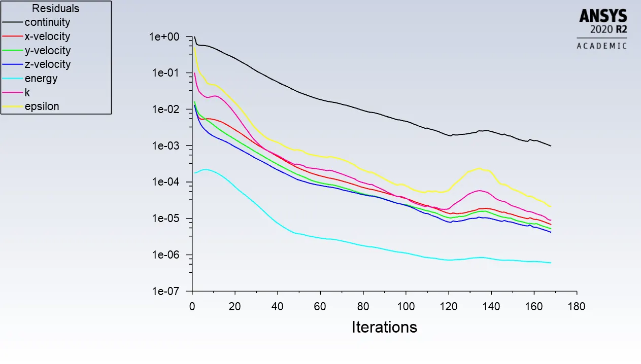
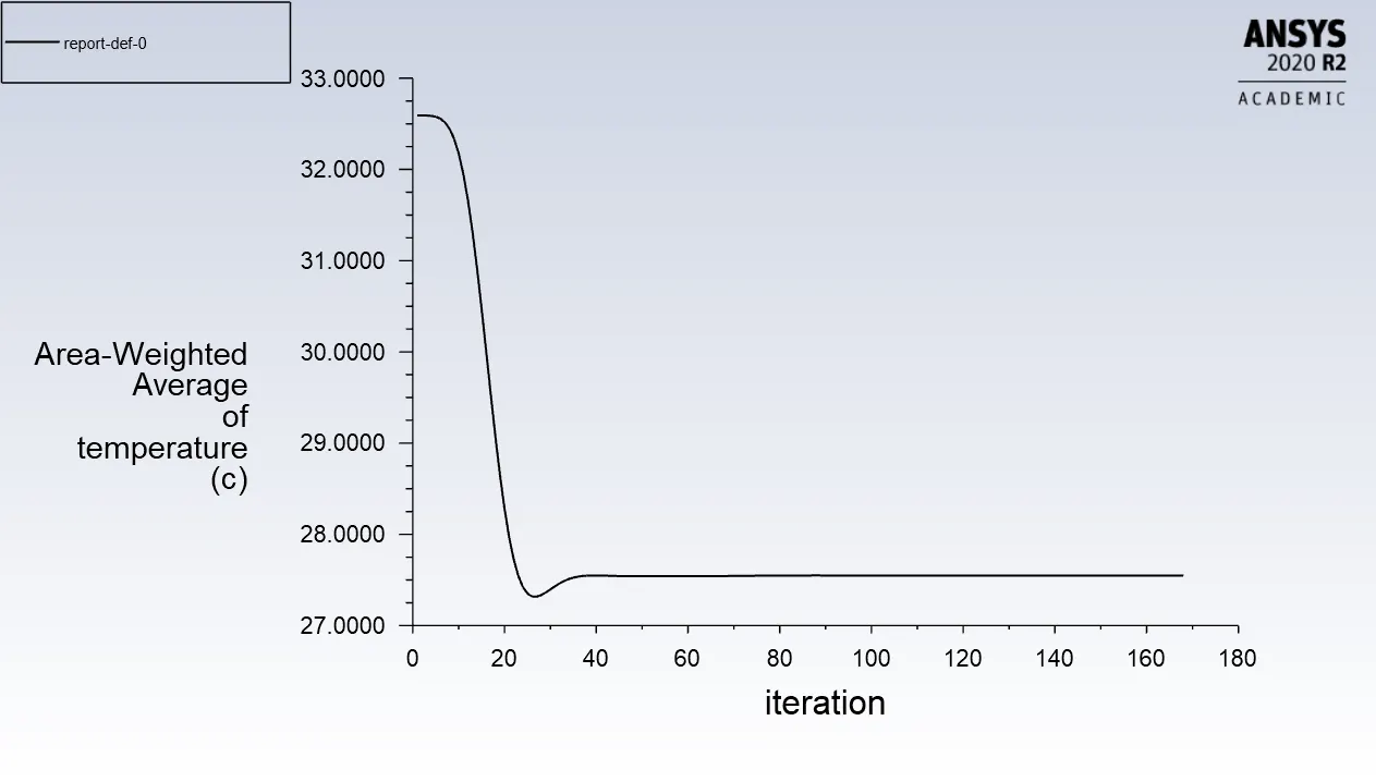
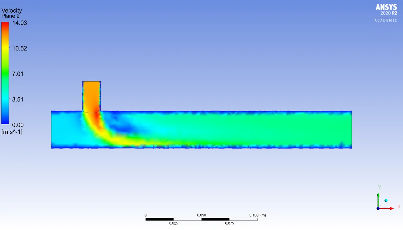
Short mixing tee for momentum ratio 4
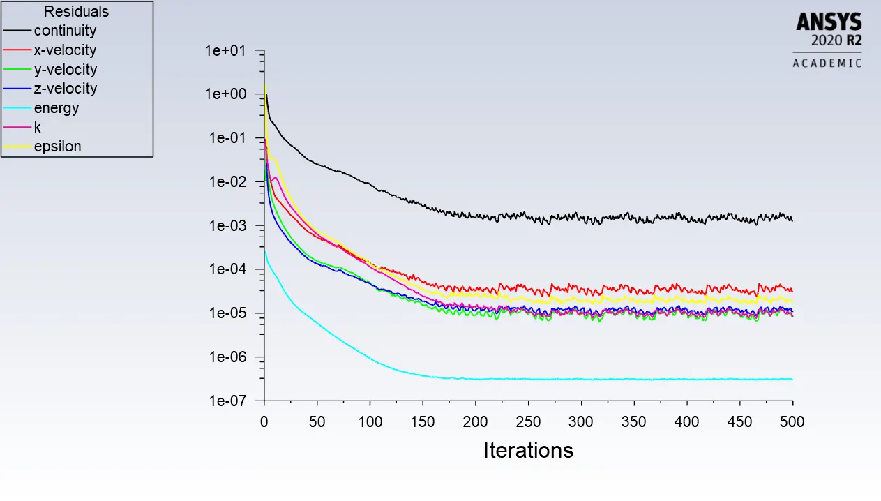
Residuals plot:
Plot showing Area weighted average of temperature to number of iterations:
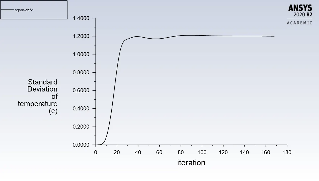
Plot showing Standard deviation of temperature to number of iterations:
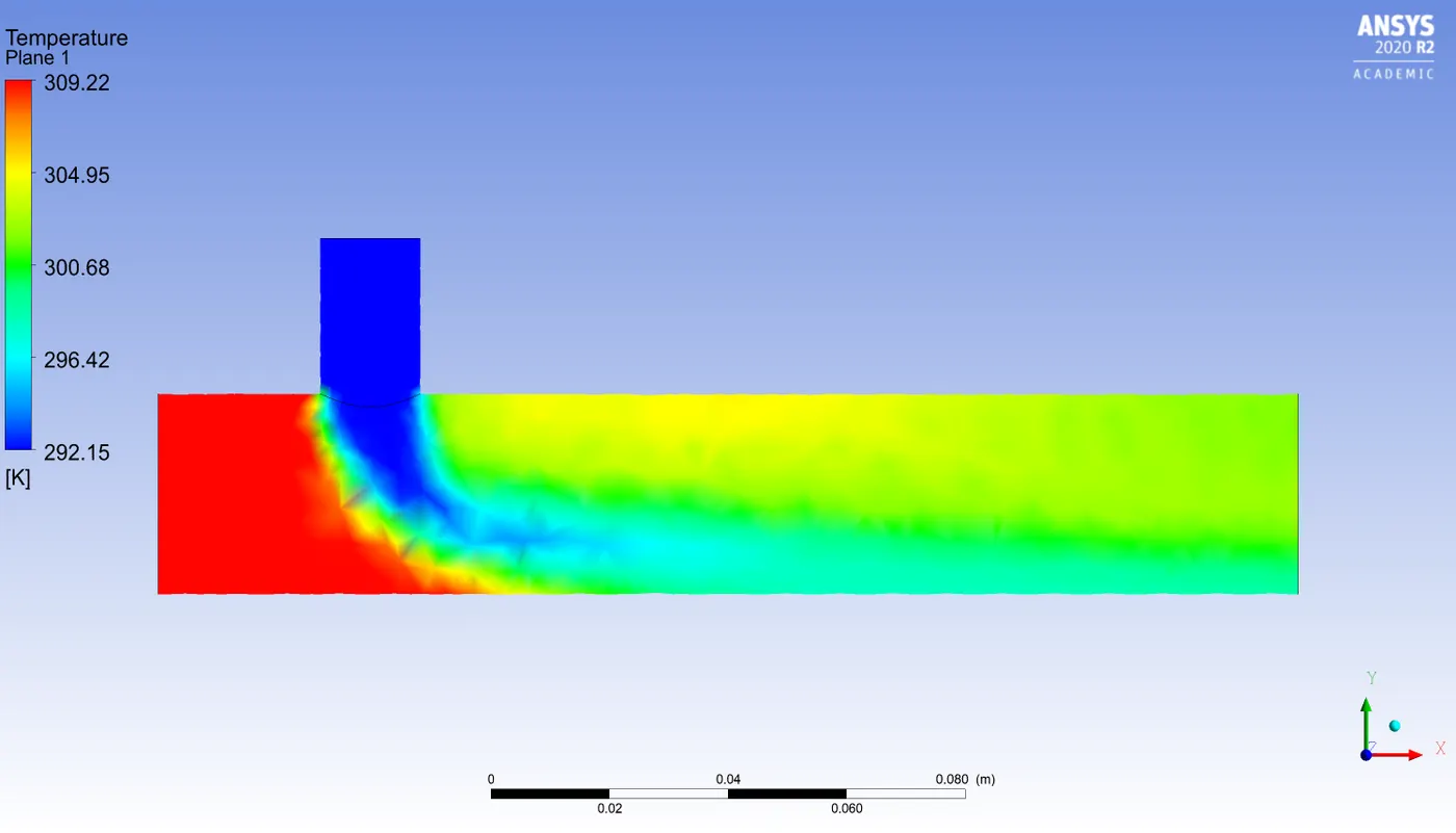
Temperature contour plot:
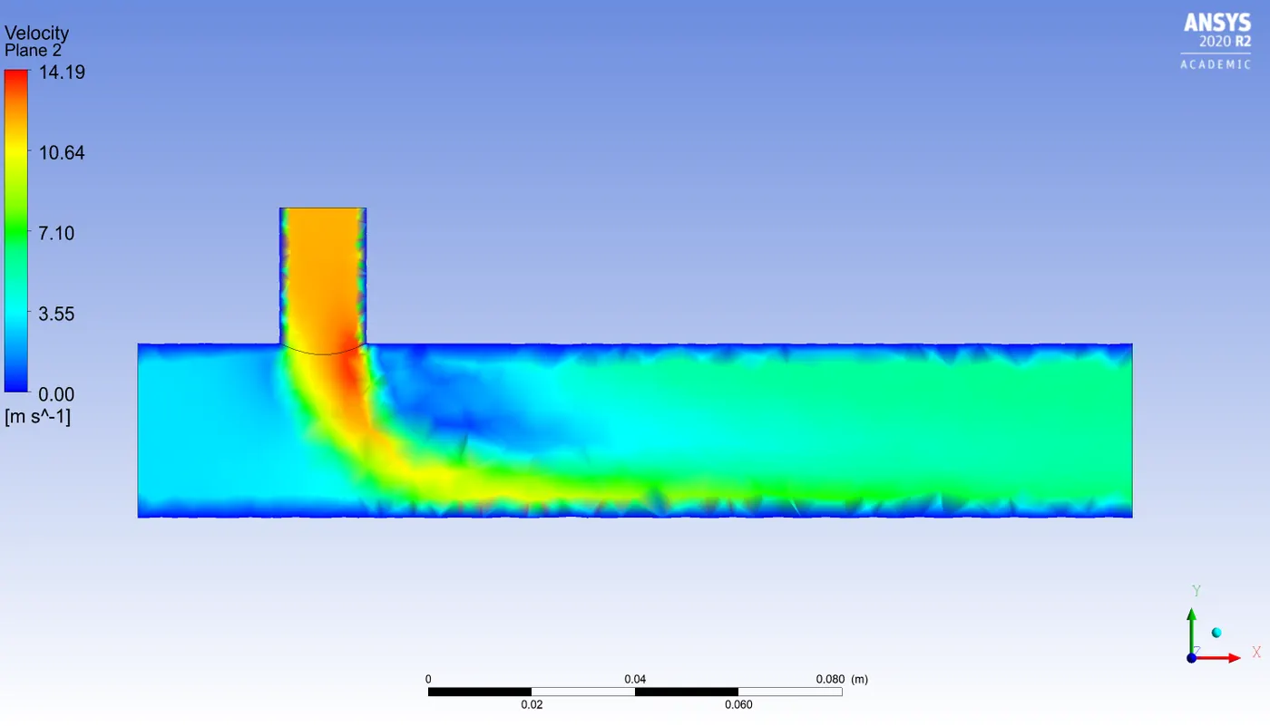
Velocity contour plot:
Long mixing tee for momentum ratio 2
Residuals plot:
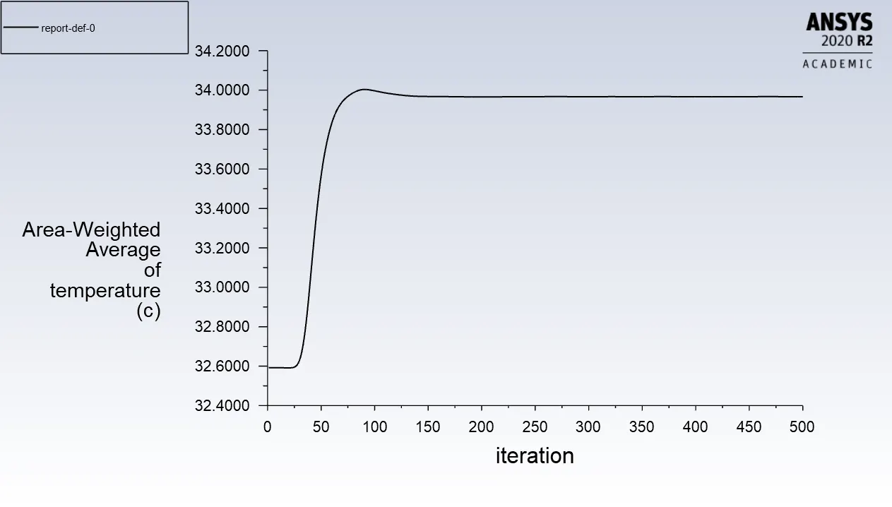
Plot showing Area weighted average of temperature to number of iterations:
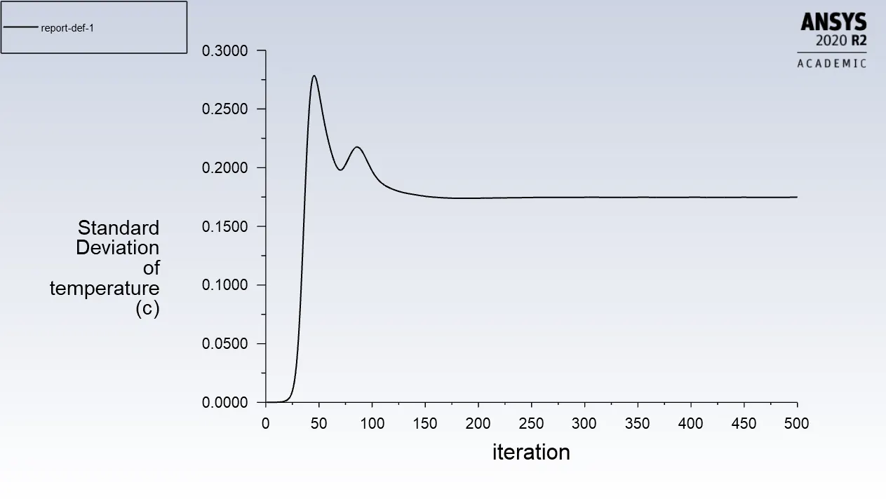
Plot showing Standard deviation of temperature to number of iterations:
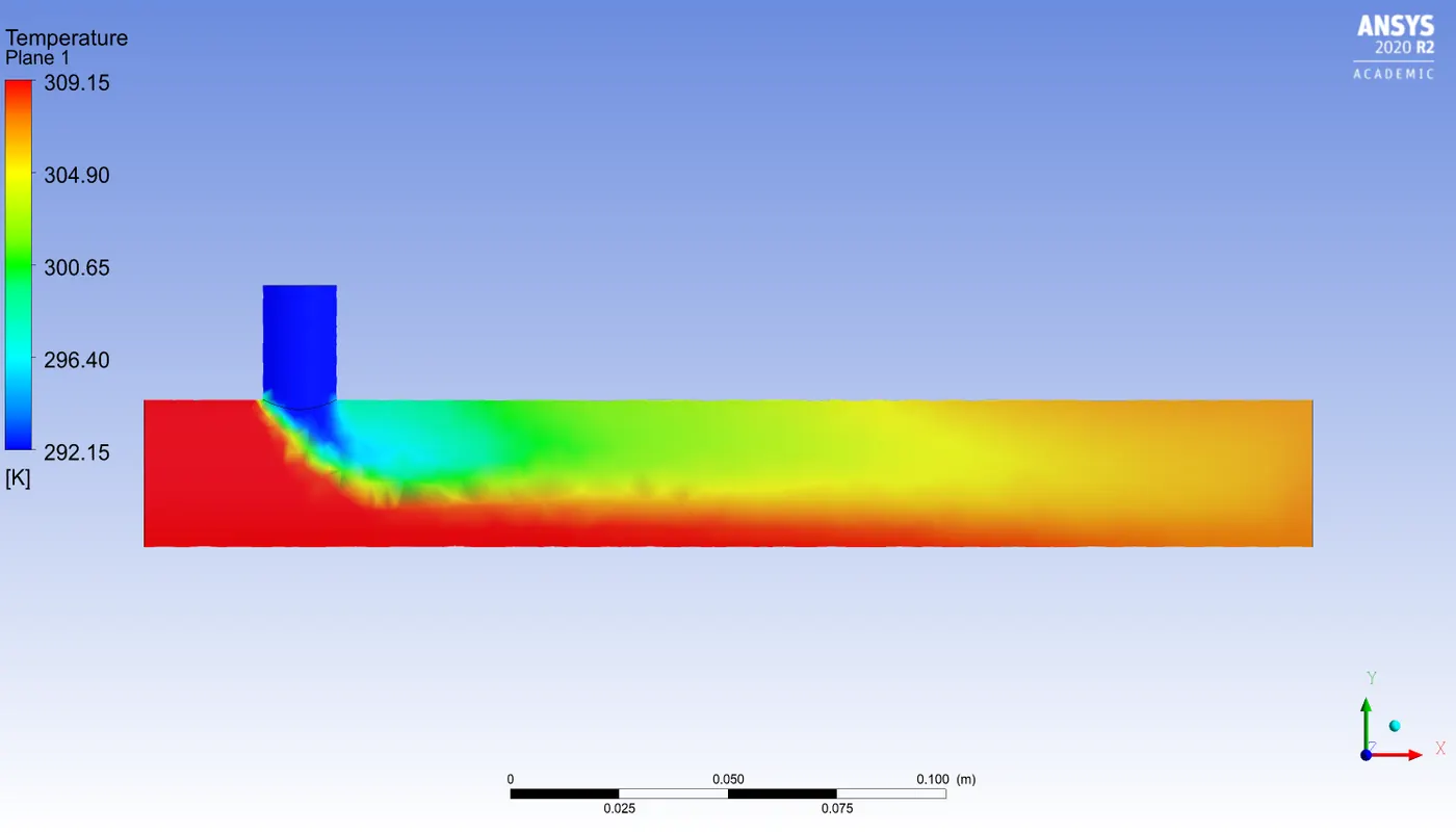
Temperature contour plot
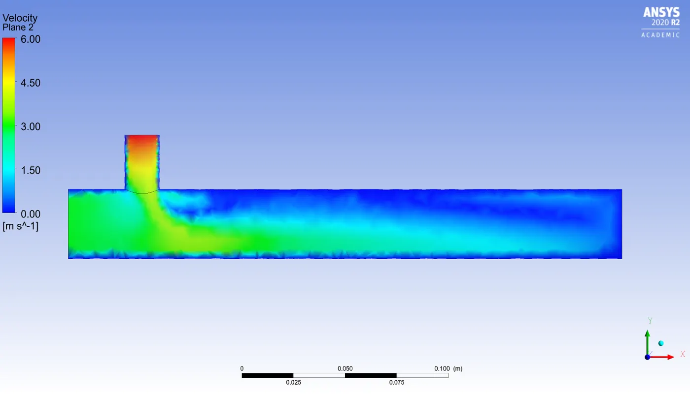
Velocity contour plot
Long mixing tee for momentum ratio 4
Residuals plot
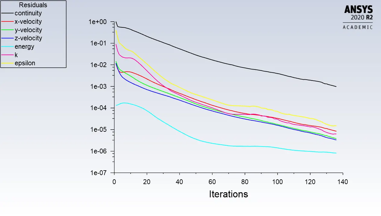
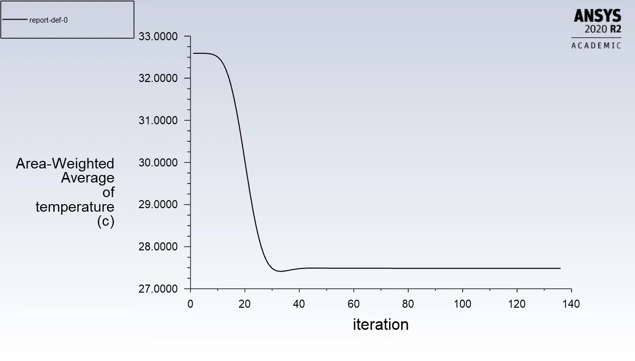
Plot showing Area weighted average of temperature to number of iterations:
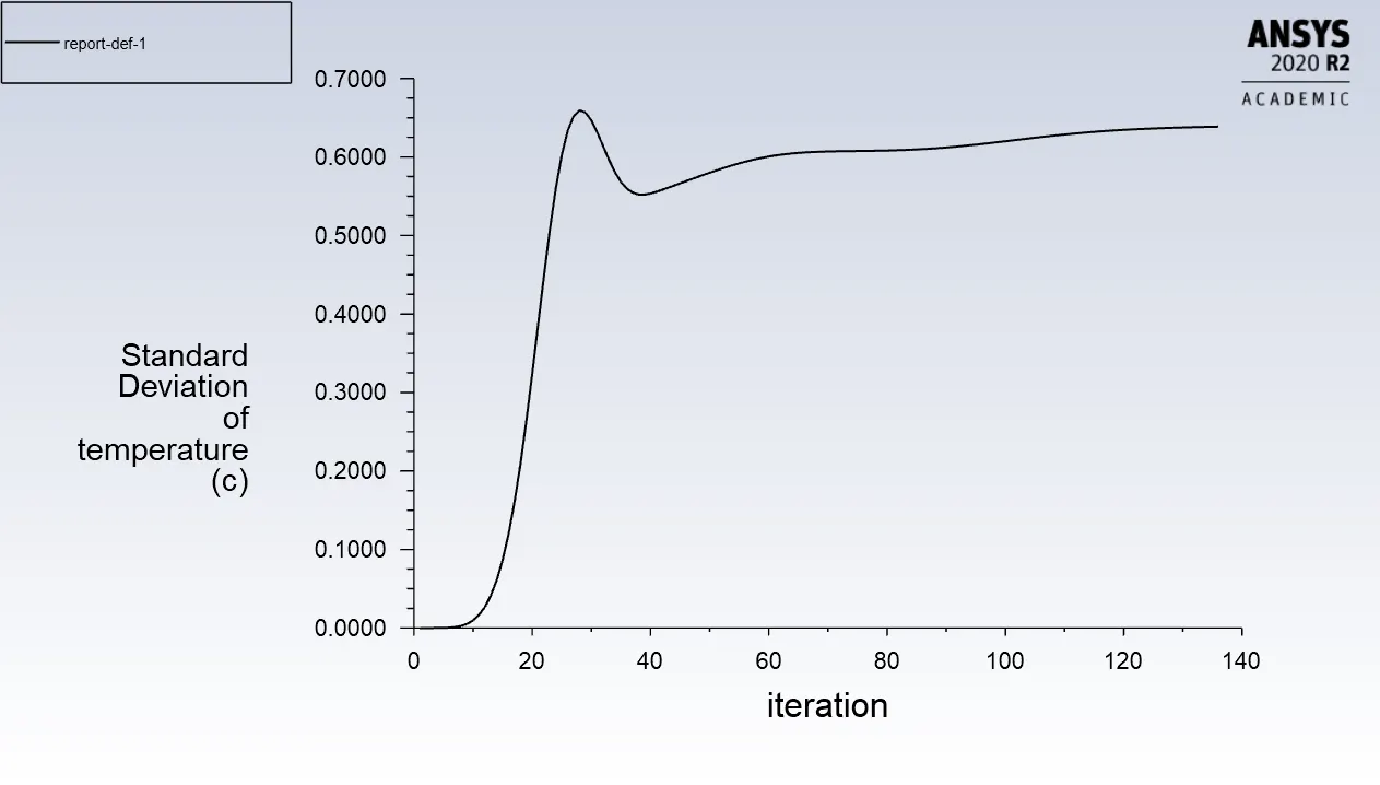
Plot showing Standard deviation of temperature to number of iterations:
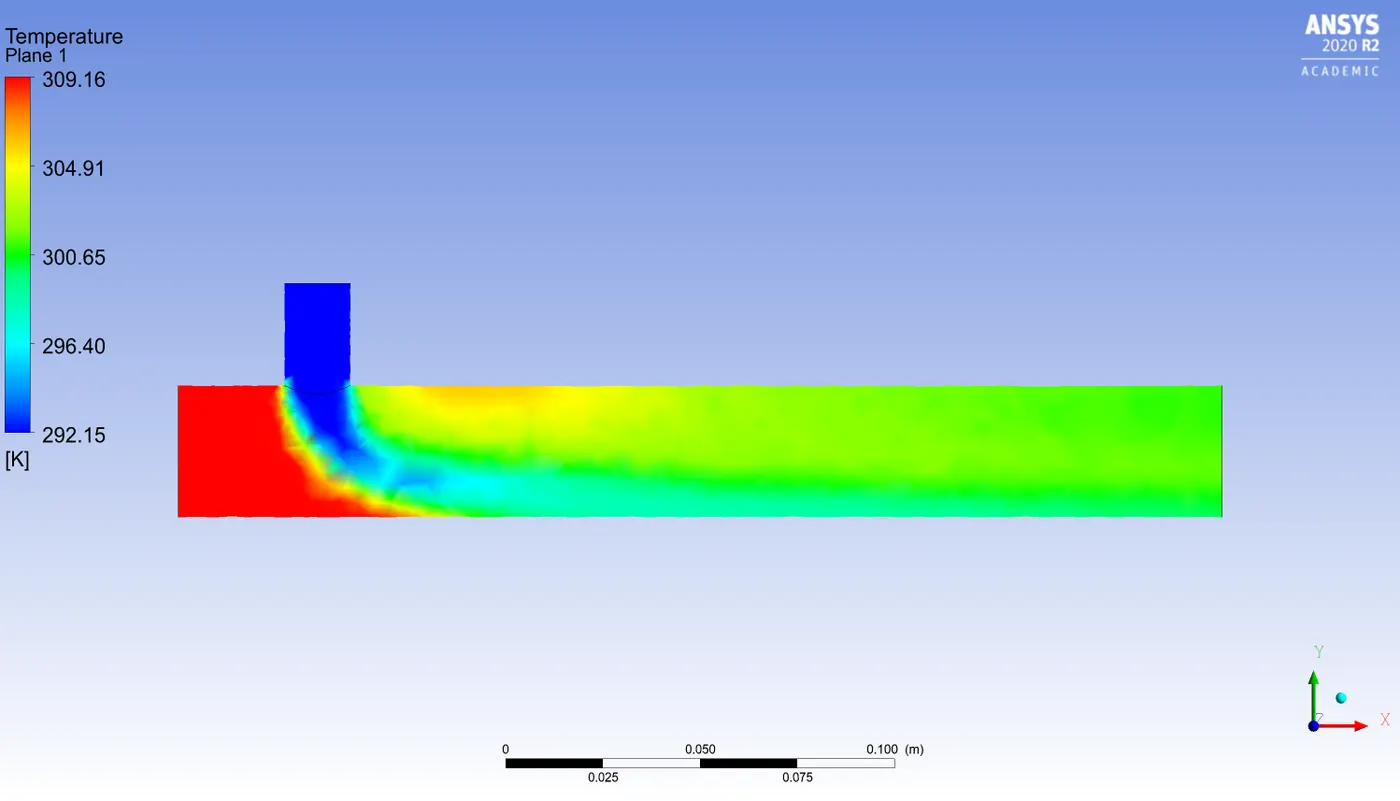
Temperature contour plot:
Velocity contour plot:
RESULT AND CONCLUSION
From the above simulations we can get the following results:
| CASE | Nodes | Elements | Max. Temp. at outlet in degree celsius | Max. Velocity reached in the mixing tee in m/s | Average Velocity in the mixing tee in m/s |
| SHORT MR 2 | 2837 | 12760 | 34.125 | 8.406 | 4.61 |
| SHORT MR 4 | 2837 | 12760 | 29.443 | 16.589 | 7.20 |
| LONG MR 2 | 3495 | 15689 | 34.316 | 6.158 | 2.25 |
| LONG MR 4 | 3495 | 15689 | 28.472 | 15.457 | 6.93 |
Where MR - momentum ratio
Conclutions from the observations made:
- It can be observed that the number of mesh nodes are more in the long tee than short tee since it has larger volume.
- The cooling effect at the end of the mixing tee is much better in the longer tee compared to shorter ones.
- The higher the moomentum factor better will be the cooling effect
- Both the average and the maximum velocity in the longer tee is less compared to the shorter tee