Week 11 - Simulation of Flow through a pipe in OpenFoam
Flow through a pipe in OpenFOAM
Principle:
The flow through a pipe works on the basis of Hagen–Poiseuille Equation which is a fluidic law to calculate flow pressure drop in a long cylindrical pipe and it was derived separately by Poiseuille and Hagen. Here let us consider a incompressible Newtonian fluid is flowing through a pipe.
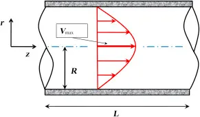
Let the length of the pipe be - L
Velocity at the center of the pipe being maximum be - Vm
Dynamic Viscosity of the fluid - `mu`
Radius of the pipe - R
Diameter of the pipe - D
Area of cross section of pipe be - A
Density of the fluid - `rho`
Mean velocity of the fluid - v
Reynold's number - Re
`v = (mu * Re) / ( rho * D)` -------------(1)
Pressure diffrence between the ends of the pipe iis given by
`Delta p = (8*mu*L*Q)/ A^2` -----------(2)
Analytical calculation:
Let us consider the following parameters :
R = 50 mm
D = 100 mm = 0.1 m
A = 0.031415 `m^2`
The fluid considered is water and all of it's properties are taken at room temperature(25deg. C)
`rho` = 997 `(Kg)/ m^3`
`mu` = `8.9*10^-4`Pa.s
Since the flow is assumed to be laminar flow, the Reynold's number is <2300, hence consider,
Re = 400
Substituting the above values to equation (1),
we get the mean velocity to be
v = 0.0035707 m/s
Analytical maximum velocity Vmax = v * 2
Vmax = 0.007141
To measure the hydrodynamic length
L = 0.006 * Re * D
L = 0.24 m
wdege angle `theta` = 3
In order to simulate a flow through an open pipe, let us consider a portion of the pipe in the form of axisymmetric wedge. This wedge has a height equal to radius of the pipe and length equal to that of the pipe and wedge angle is less than 5 degrees. Here we have considered the wedge angle to be 3 degrees, smaller the angle finer is the boundary layer and the result will be closer to actual solution.
Vertices numbering of the wedge:
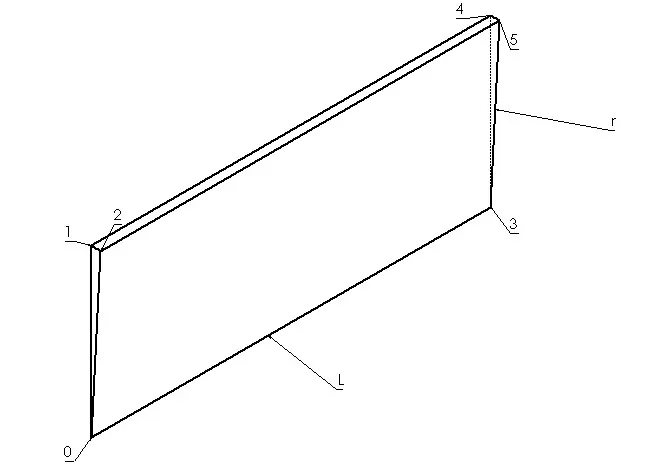
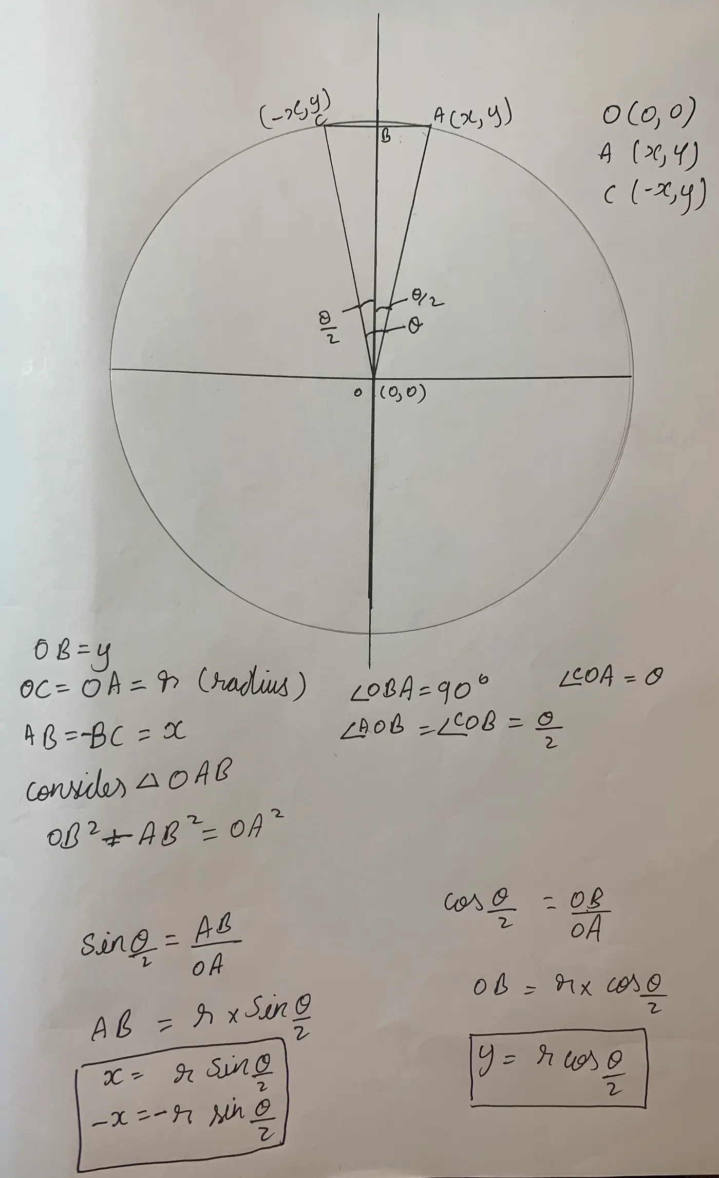
To find the vertices co-ordinates, consider the face of the pipe inlet and wedge to be considered be given by triangle OAC, and the wedge angle is a very small angle, <5degrees denoted by `theta`. The image below shows the calculation to determine vertices co-ordinates of the wedge:
Matlab code to generate blockMeshDict:
The program code below generates the blockMeshhDict file for a given radius of the pipe. The angle considered is 3 deegrees and the grading factor is 1 along all the axes, it can be changed as per requirement.
clear all
close all
clc

%Radius in meters
r = 0.05;
%Diameter in meters
d = 0.1;
%Wedge angle in degrees
theta = 3;
%Reynold's number
Re = 400;
%Length of the pipe
L = (0.006*Re*d);
%Dynamic viscosity
mu = 0.00089;
%Density
rho = 997;
%number of mesh points along the length of the pipe
nl = 100;
%number of mesh points along the radius of the pipe
nr = 50;
%grading scheme along respective axis
x = 1;
y = 1;
z = 1;
%vertices
v0 = [ 0 0 0];
v1 = [0  r*cosd(theta/2) -r*sind(theta/2) ];
v2 = [0  r*cosd(theta/2) r*sind(theta/2) ];
v3 = [L 0 0];
v4 = [L  r*cosd(theta/2) -r*sind(theta/2) ];
v5 = [L  r*cosd(theta/2)  r*sind(theta/2)];

f1 = fopen('blockMeshDict.txt','w');

fprintf(f1,'FoamFile\n');
fprintf(f1,'{\n');
fprintf(f1,'     version    2.0;\n');
fprintf(f1,'     format     ascii;\n');
fprintf(f1,'     class      dictionary;\n');
fprintf(f1,'     object     blockMeshDict;\n');
fprintf(f1,'}\n');
fprintf(f1,'//**************************************// \n\n');
fprintf(f1,'convertToMeters 1;\n\n');
fprintf(f1,'vertices\n');
fprintf(f1,'(\n\t');
fprintf(f1,'(%.7f %.7f %.7f) //0 \n\t',v0(1),v0(2),v0(3));
fprintf(f1,'(%.7f %.7f %.7f) //1 \n\t',v1(1),v1(2),v1(3));
fprintf(f1,'(%.7f %.7f %.7f) //2 \n\t',v2(1),v2(2),v2(3));
fprintf(f1,'(%.7f %.7f %.7f) //3 \n\t',v3(1),v3(2),v3(3));
fprintf(f1,'(%.7f %.7f %.7f) //4 \n\t',v4(1),v4(2),v4(3));
fprintf(f1,'(%.7f %.7f %.7f) //5 \n\n',v5(1),v5(2),v5(3));
fprintf(f1,');\n\n');

fprintf(f1,'blocks\n');
fprintf(f1,'(\n\t');
fprintf(f1,'hex ( 0 1 2 0 3 4 5 3) (%d 1 %d) simpleGrading (%.2f %.2f %.2f)\n',nl,nr,x,y,z);
fprintf(f1,');\n\n');

fprintf(f1,'edges\n');
fprintf(f1,'(\n\t');
fprintf(f1,'arc 2 1 (0 %.3f 0)\n\t',r);
fprintf(f1,'arc 5 4 (%.3f %.3f 0)\n',L,r);
fprintf(f1,');\n\n');

fprintf(f1,'boundary\n');
fprintf(f1,'(\n\t');

fprintf(f1,'axis\n\t');
fprintf(f1,'{\n\t\t');
fprintf(f1,'type empty;\n\t\t');
fprintf(f1,'faces\n\t\t');
fprintf(f1,'(\n\t\t\t');
fprintf(f1,'(0 3 3 0)\n\t\t');
fprintf(f1,');\n\t');
fprintf(f1,'}\n\n\t');

fprintf(f1,'inlet\n\t');
fprintf(f1,'{\n\t\t');
fprintf(f1,'type patch;\n\t\t');
fprintf(f1,'faces\n\t\t');
fprintf(f1,'(\n\t\t\t');
fprintf(f1,'(0 2 1 0)\n\t\t');
fprintf(f1,');\n\t');
fprintf(f1,'}\n\n\t');

fprintf(f1,'outlet\n\t');
fprintf(f1,'{\n\t\t');
fprintf(f1,'type patch;\n\t\t');
fprintf(f1,'faces\n\t\t');
fprintf(f1,'(\n\t\t\t');
fprintf(f1,'(3 4 5 3)\n\t\t');
fprintf(f1,');\n\t');
fprintf(f1,'}\n\n\t');

fprintf(f1,'fixedWalls\n\t');
fprintf(f1,'{\n\t\t');
fprintf(f1,'type wall;\n\t\t');
fprintf(f1,'faces\n\t\t');
fprintf(f1,'(\n\t\t\t');
fprintf(f1,'(1 2 5 4)\n\t\t');
fprintf(f1,');\n\t');
fprintf(f1,'}\n\n\t');

fprintf(f1,'front\n\t');
fprintf(f1,'{\n\t\t');
fprintf(f1,'type wedge;\n\t\t');
fprintf(f1,'faces\n\t\t');
fprintf(f1,'(\n\t\t\t');
fprintf(f1,'(0 3 5 2)\n\t\t');
fprintf(f1,');\n\t');
fprintf(f1,'}\n\n\t');

fprintf(f1,'back\n\t');
fprintf(f1,'{\n\t\t');
fprintf(f1,'type wedge;\n\t\t');
fprintf(f1,'faces\n\t\t');
fprintf(f1,'(\n\t\t\t');
fprintf(f1,'(0 1 4 3)\n\t\t');
fprintf(f1,');\n\t');
fprintf(f1,'}\n');
fprintf(f1,');\n\n');

fprintf(f1,'mergePatchPairs\n\n');
fprintf(f1,'(\n\n');
fprintf(f1,');\n\n');

fprintf(f1,'//**************************************//');

fclose(f1)
blockMeshDict file:
The blockmeshdict file generated by the matlab code is given below
FoamFile
{
     version    2.0;
     format     ascii;
     class      dictionary;
     object     blockMeshDict;
}
//**************************************//

convertToMeters 1;

vertices
(
	(0.0000000 0.0000000 0.0000000) //0
	(0.0000000 0.0499829 -0.0013088) //1
	(0.0000000 0.0499829 0.0013088) //2
	(0.2400000 0.0000000 0.0000000) //3
	(0.2400000 0.0499829 -0.0013088) //4
	(0.2400000 0.0499829 0.0013088) //5

);

blocks
(
	hex ( 0 1 2 0 3 4 5 3) (100 1 50) simpleGrading (1.000000 1.000000 1.000000)
);

edges
(
	arc 2 1 (0 0.050 0)
	arc 5 4 (0.240 0.050 0)
);

boundary
(
	axis
	{
		type empty;
		faces
		(
			(0 3 3 0)
		);
	}

	inlet
	{
		type patch;
		faces
		(
			(0 2 1 0)
		);
	}

	outlet
	{
		type patch;
		faces
		(
			(3 4 5 3)
		);
	}

	fixedWalls
	{
		type wall;
		faces
		(
			(1 2 5 4)
		);
	}

	front
	{
		type wedge;
		faces
		(
			(0 3 5 2)
		);
	}

	back
	{
		type wedge;
		faces
		(
			(0 1 4 3)
		);
	}
);

mergePatchPairs

(

);

//**************************************//
controlDict file:
/*--------------------------------*- C++ -*----------------------------------*\
  =========                 |
  \\      /  F ield         | OpenFOAM: The Open Source CFD Toolbox
   \\    /   O peration     | Website:  https://openfoam.org
    \\  /    A nd           | Version:  8
     \\/     M anipulation  |
\*---------------------------------------------------------------------------*/
FoamFile
{
    version     2.0;
    format      ascii;
    class       dictionary;
    location    "system";
    object      controlDict;
}
// * * * * * * * * * * * * * * * * * * * * * * * * * * * * * * * * * * * * * //

application     icoFoam;

startFrom       startTime;

startTime       0;

stopAt          endTime;

endTime         10;

deltaT          1e-3;

writeControl    timeStep;

writeInterval   20;

purgeWrite      0;

writeFormat     ascii;

writePrecision  6;

writeCompression off;

timeFormat      general;

timePrecision   6;

runTimeModifiable true;


// ************************************************************************* //
Velocity boundary condition:
/*--------------------------------*- C++ -*----------------------------------*\
  =========                 |
  \\      /  F ield         | OpenFOAM: The Open Source CFD Toolbox
   \\    /   O peration     | Website:  https://openfoam.org
    \\  /    A nd           | Version:  8
     \\/     M anipulation  |
\*---------------------------------------------------------------------------*/
FoamFile
{
    version     2.0;
    format      ascii;
    class       volVectorField;
    object      U;
}
// * * * * * * * * * * * * * * * * * * * * * * * * * * * * * * * * * * * * * //

dimensions      [0 1 -1 0 0 0 0];

internalField   uniform (0.0035707 0 0);

boundaryField
{
    inlet
    {
        type            fixedValue;
        value		 $internalField;
    }

    fixedWalls
    {
        type            fixedValue;
        value           uniform (0 0 0);
    }
    outlet
    {
        type            zeroGradient;

    }

    axis
    {
        type            empty;
    }
    front
    {
        type            wedge;
    }
    back
    {
        type            wedge;
    }
}

// ************************************************************************* //
Pressure boundary condition:
/*--------------------------------*- C++ -*----------------------------------*\
  =========                 |
  \\      /  F ield         | OpenFOAM: The Open Source CFD Toolbox
   \\    /   O peration     | Website:  https://openfoam.org
    \\  /    A nd           | Version:  8
     \\/     M anipulation  |
\*---------------------------------------------------------------------------*/
FoamFile
{
    version     2.0;
    format      ascii;
    class       volScalarField;
    object      p;
}
// * * * * * * * * * * * * * * * * * * * * * * * * * * * * * * * * * * * * * //

dimensions      [0 2 -2 0 0 0 0];

internalField   uniform 0;

boundaryField
{
    inlet
    {
        type            zeroGradient;
    }

    fixedWalls
    {
        type            zeroGradient;
    }
    outlet
    {
        type            zeroGradient;
        value           $internalField;
    }

    axis
    {
        type            empty;
    }
    front
    {
        type            wedge;
    }
    back
    {
        type            wedge;
    }
}

// ************************************************************************* //
Transport properties:
/*--------------------------------*- C++ -*----------------------------------*\
  =========                 |
  \\      /  F ield         | OpenFOAM: The Open Source CFD Toolbox
   \\    /   O peration     | Website:  https://openfoam.org
    \\  /    A nd           | Version:  8
     \\/     M anipulation  |
\*---------------------------------------------------------------------------*/
FoamFile
{
    version     2.0;
    format      ascii;
    class       dictionary;
    location    "constant";
    object      transportProperties;
}
// * * * * * * * * * * * * * * * * * * * * * * * * * * * * * * * * * * * * * //

nu              [0 2 -1 0 0 0 0] 0.0000089267;


// ************************************************************************* //
mesh:
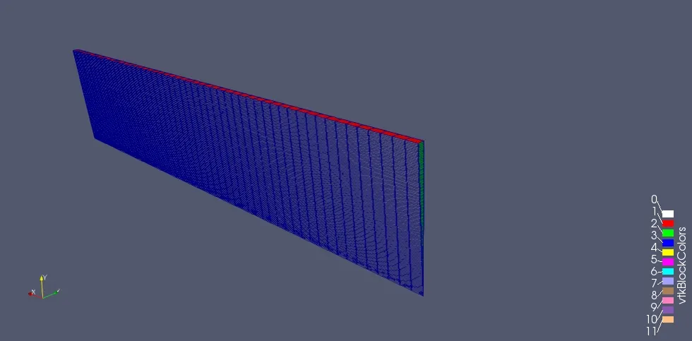
The mesh generated is of grading 1 in all direction.
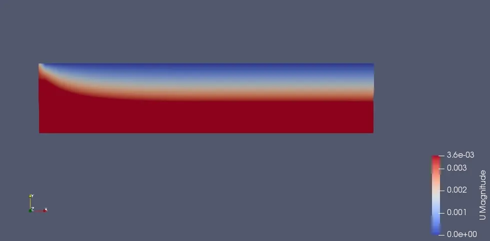
Velocity:
The image below shows the velocity contour inside the pipe
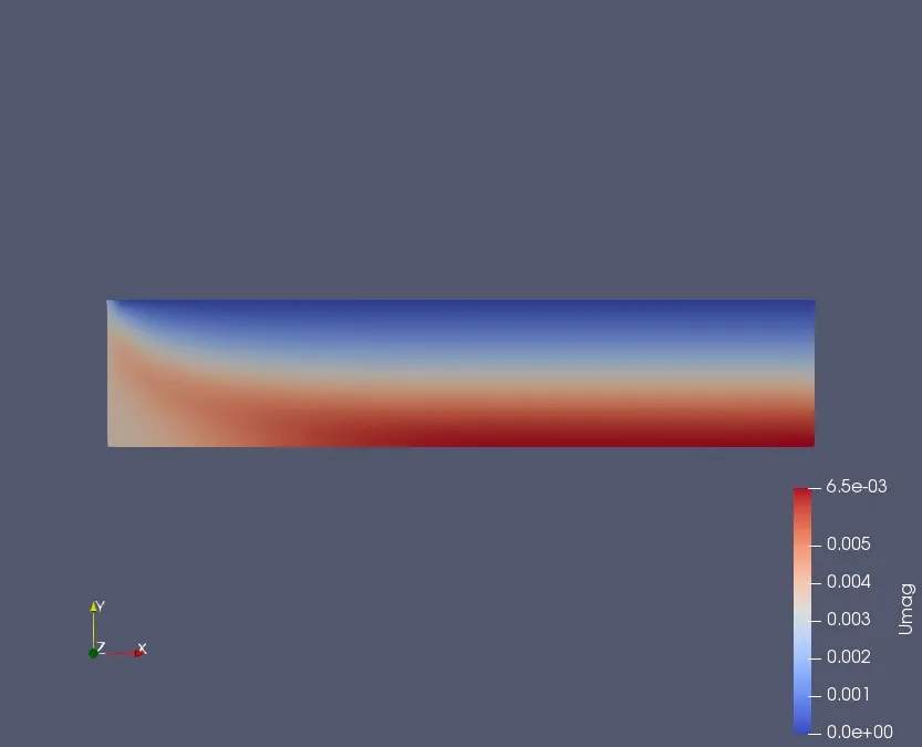
Fully developed profile:
The image below shows the velocity contour inside the pipe after the vector field inside the pipe calculated
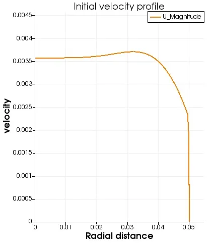
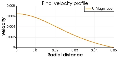
Velocity plots
In the images below we can see the plot of the velocity profile at the inlet and the outlet and it can be observed that the velocity is smoothened out the the end and considering that the flow is laminar, it checks out with Hagen-Poiseuille's flow equation and it can be observed the maximum velocity is at the centre and the velocity decreases as we move towards the walls of the pipe.
pressure plot:
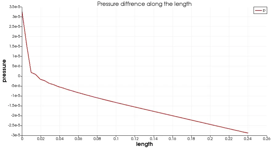
The image below shows a plot on how the pressure changes inside the pipe after the flow is simulated along the length of the pipe. We can see how the pressure at the entrance is higher than that of the outlet
Shear stress plot:
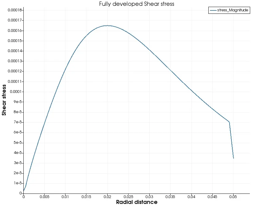
The image below shows the plot on how the shear stress on the fluid flowing is varying along the radial length of the pipe. It can be observed that it gradually increases while moving from the centre of the pipe radially. As we start to approach the pipe wall the shear stress increases.
Analytical to simulation comparison:
| Analytical | Simulation | Diffrence | Percentage error | |
| Maximum Velocity | 0.007141 | 0.006505 | 0.000636 | 8.9% |
By comparing the maximum velocity values obtained from simulation and analytical calculation, we can see that the simulation result is close to analytical calculations with an error of about 9%.