Steady Vs Unsteady flow over a cylinder
Aim:
The aim of this project is to study a two dimensiona flow of a user specified fluid over a 2-D cylinder on a plane for varying Reynolds number.
Introduction:
When a fluid is made to flow over a cylinder vortex is produced. A vortex is in the process of formation near the top of the cylinder surface. Below and to the right of the first vortex is another vortex which was formed and shed a short period before. Thus, the flow process in the wake of a cylinder or tube involves the formation and shedding of vortices alternately from one side and then the other. This phenomenon is of major importance in engineering design because the alternate formation and shedding of vortices also creates alternating forces, which occur more frequently as the velocity of the flow increases.
Von Kármán vortex street is a repeating pattern of swirling vortices, caused by a process known as vortex shedding, which is responsible for the unsteady separation of flow of a fluid around blunt bodies.
Strouhal number Sr is a dimensionless number commonly used as a measure of the predominant shedding frequency fs, where L is a characteristic length and U the freestream velocity.
`Sr = (Fs ** L ) / U`
Model geometry:
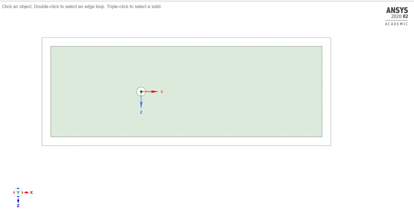
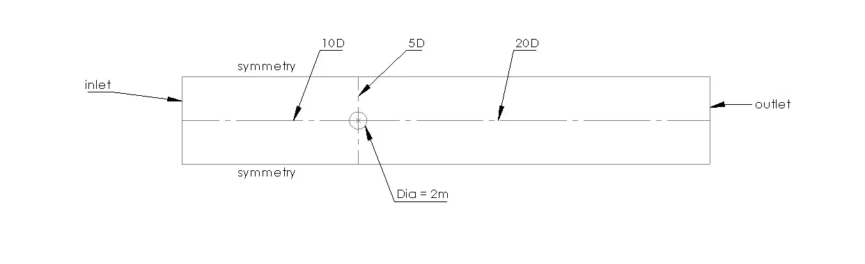
The image below shows the model created using space claim and the boundary around the cylinder is determined by the diameter of the cylinder.
Meshing:
All triangles method is used for meshing where all the mesh elements are converted to triangular from quadrilateral.
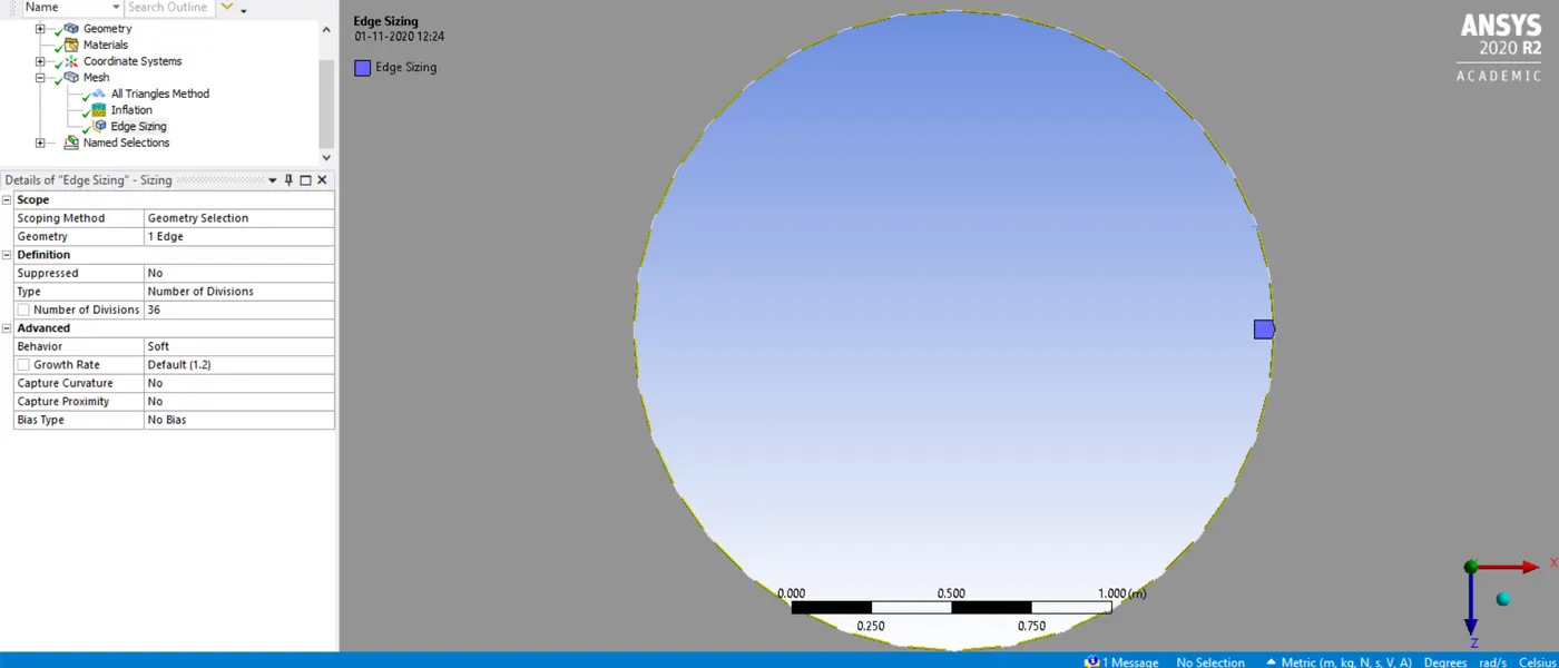
At this point the cylinder wall is more like a polygon than a circle, in order to rectify this we use the edge sizing option to smooth out the wall of the cylinder as shown in the image below
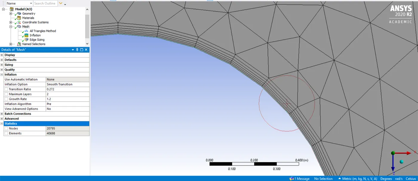
Also The edge inflation around the cylinder wall is performed to obtain smooth flow around the cylinder. The image below shows the inflation layers around the cylinder wall
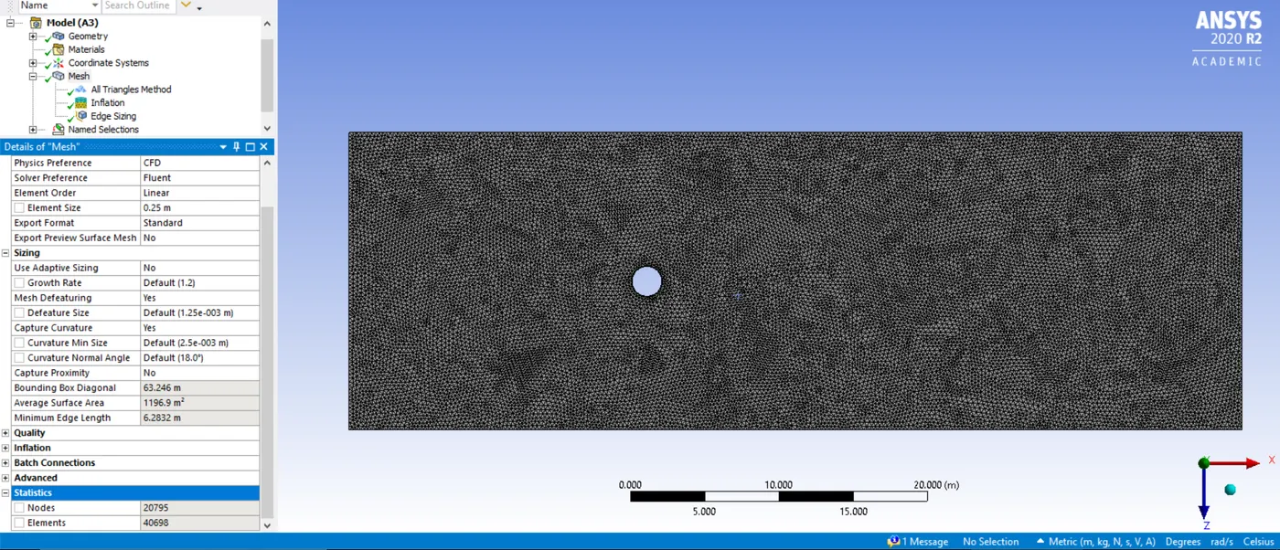
The image below shows the final mesh. As we can see that the elements are of very small size in order to capture the accurate results.
Part 1 : Steady state v/s Transient state simulation for Reynolds number 100
The Reynolds number (Re) helps predict flow patterns in different fluid flow situations and is given by
`Re = (rho**u**L)/ mu`
where:
`rho` is the density of the fluid (SI units: `(kg)/ m^3`)
u is the flow speed (m/s)
L is a characteristic linear dimension (m)
`mu` is the dynamic viscosity of the fluid (kg/(m·s))
Setup :
For the setup of the simulation we create our own fluid which has the following properties :
Density = 1 `(kg)/ m^3`
Viscosity = 0.05 Kg/(m.s)
By setting the inlet velocity of the fluid to 2.5 m/s we get the Reynolds number 100.
Laminar Viscous model is used throught this project and also the same material but in order to change the Re the inlet velocity is varied acccordingly.
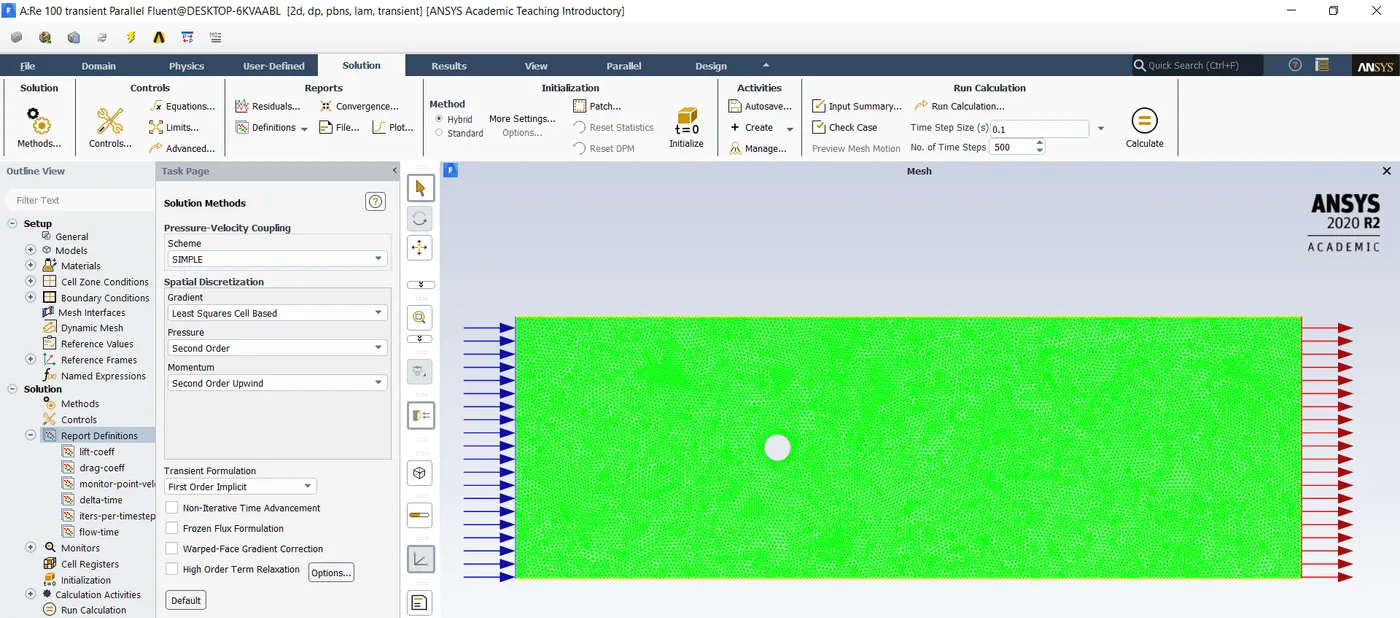
The image below shows the final setup required for the simulation.
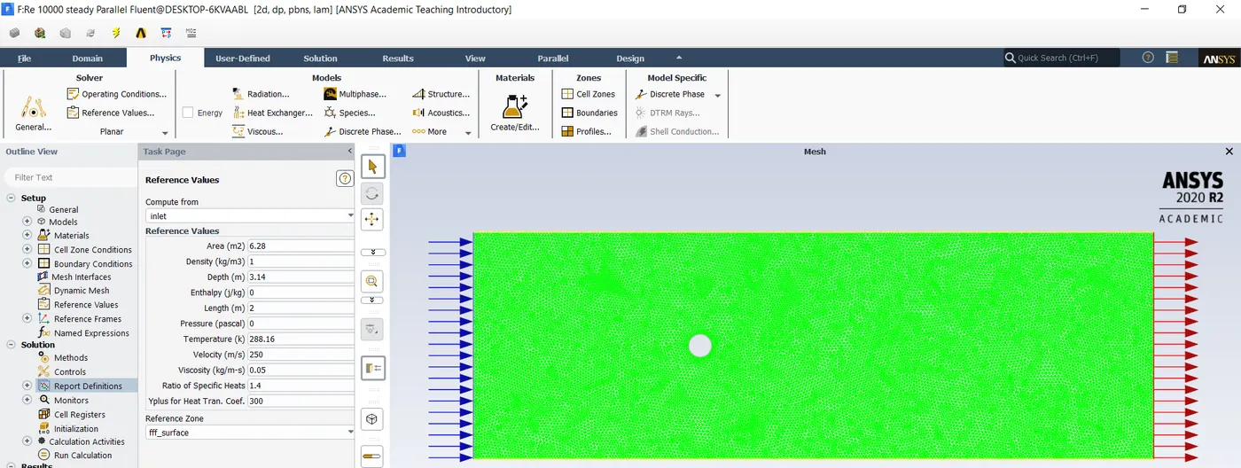
The reference values taken for the setup in order to get accurate results can be seen in the image below, as the solver has to compute from the values given at the input
Case 1 :
Pressure based solver is used with the time being transient.
Boundary conditions are given as,
inlet wall is of velocity inlet where the velocity is taken as per the situation, in this case 2.5m/s .
outlet wall is of velocity outlet where gauge pressure is 0Pa.
The reamining two sides is of symmetry condition since the flow is incompressible.
The cylinder is taken as a smooth boundary i.e. wall.
Drag coefficients and lift coefficients are reported and a monitor point behind the cylinder is allocated to measure the change in the velocity of the fluid.
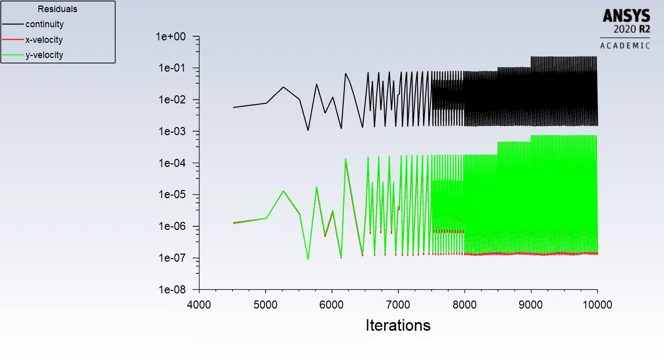
Residual plot:
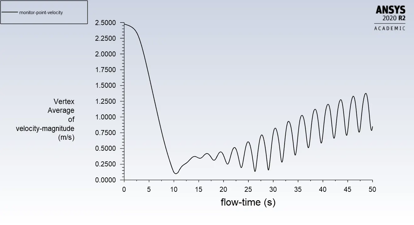
Monitor point velocity plot:
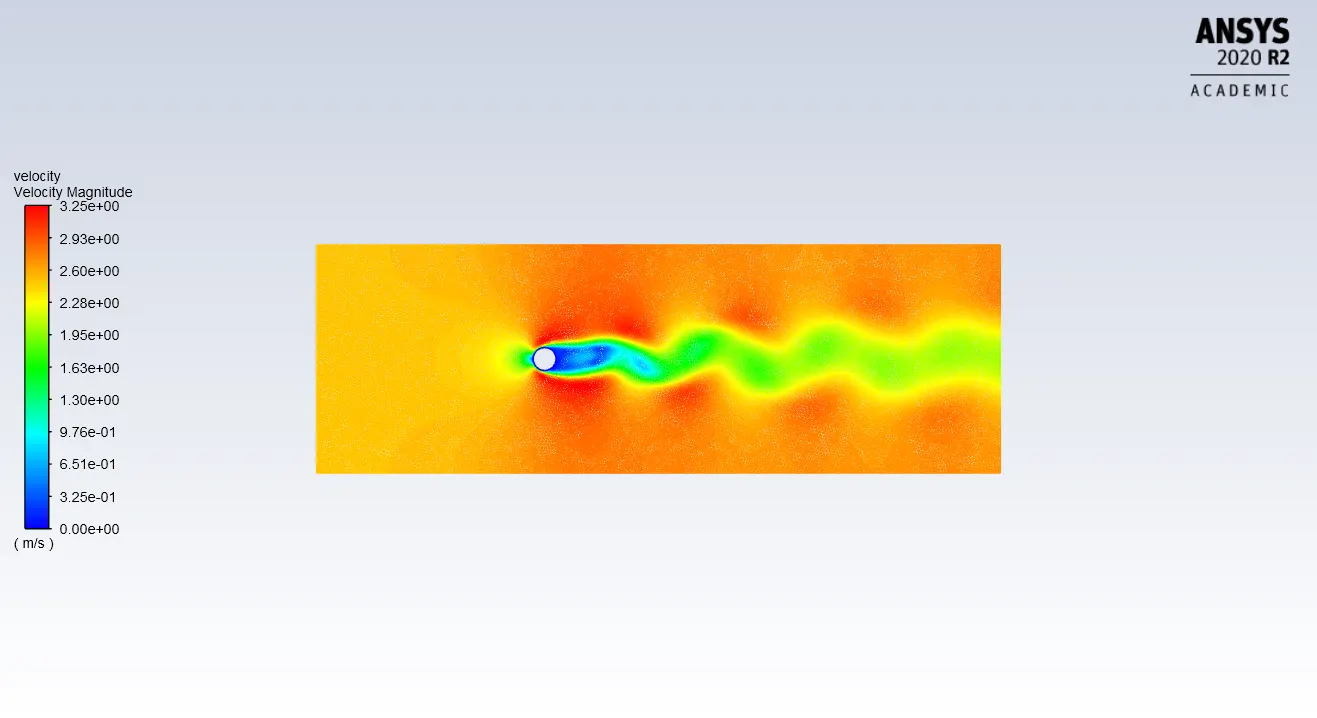
Velocity contour
Drag co efficient
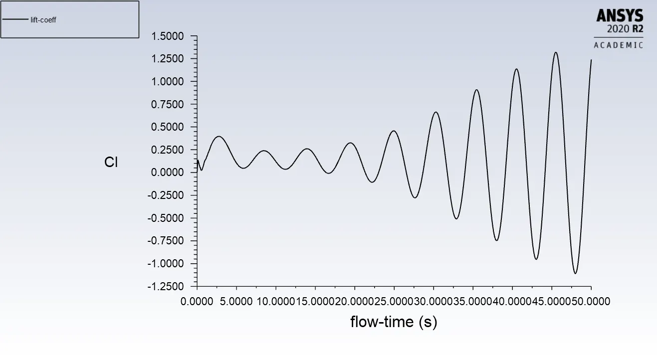
Coefficient of lift
Case 2 :
Pressure based solver is used with the time being steady.
The image below shows the final setup required for the simulation.
Boundary conditions are given as,
inlet wall is of velocity inlet where the velocity is taken as per the situation, in this case 2.5m/s .
outlet wall is of velocity outlet where gauge pressure is 0Pa.
The reamining two sides is of symmetry condition since the flow is incompressible.
The cylinder is taken as a smooth boundary i.e. wall.
Drag coefficients and lift coefficients are reported and a monitor point behind the cylinder is allocated to measure the change in the velocity of the fluid.
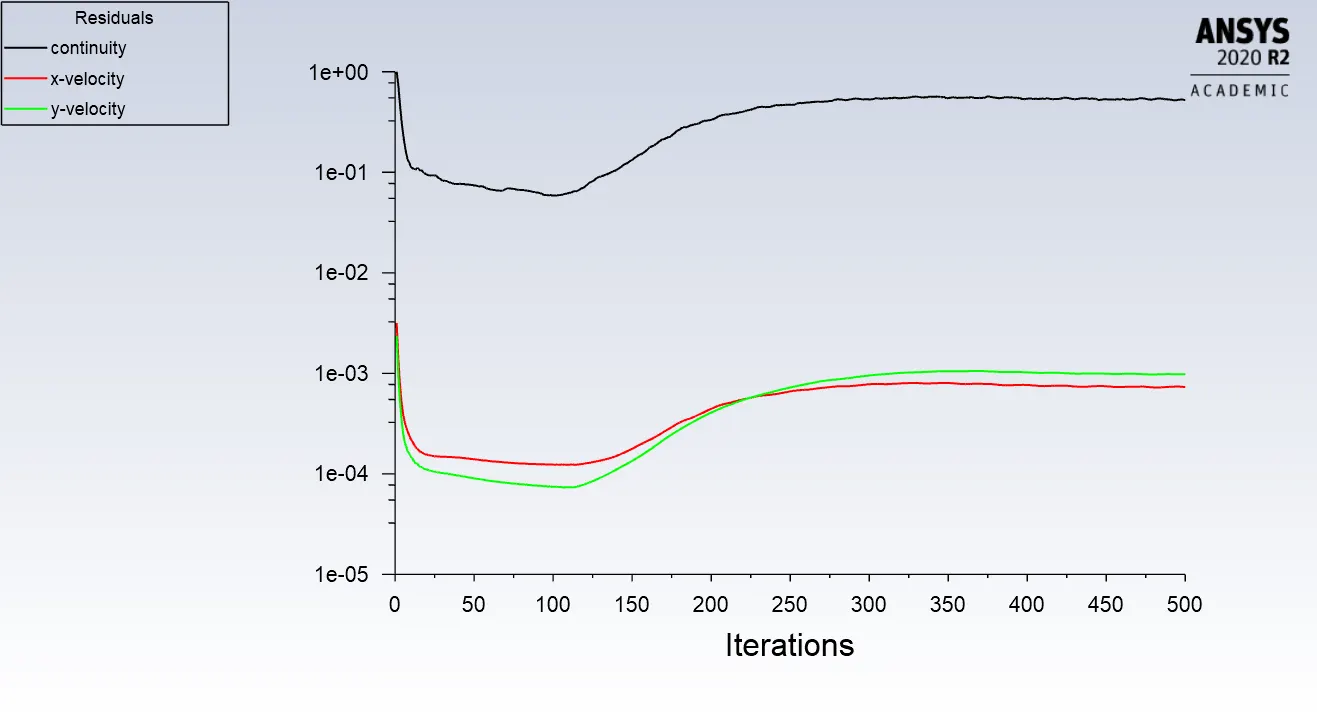
Residual plot:
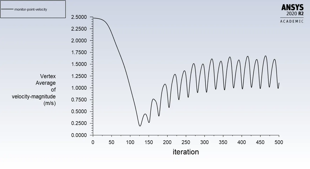
Monitor point velocity plot:
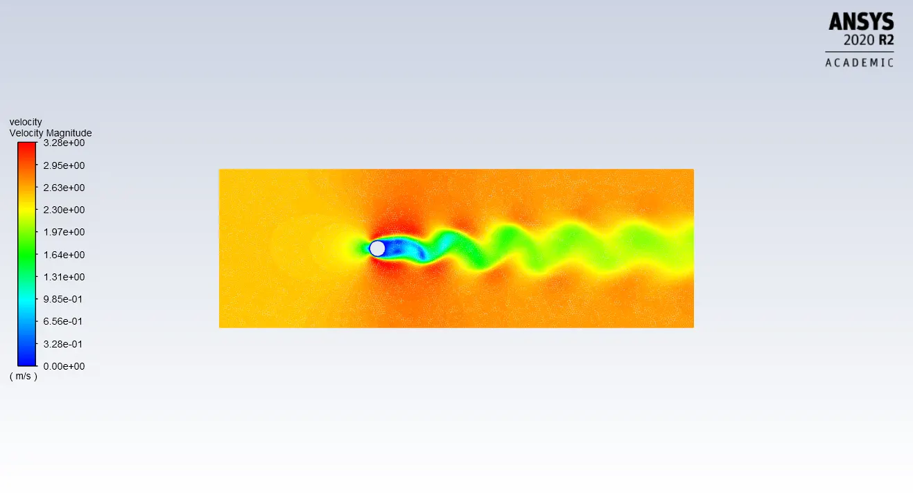
Velocity contour:
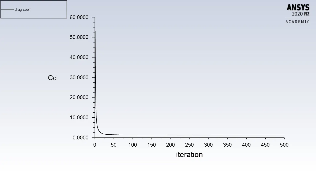
Drag coefficient plot :
Lift coefficient plot:
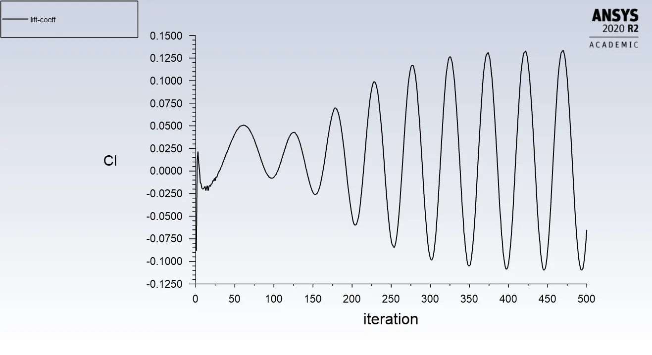
To calculate Strouhal number
`Sr = (Fs ** L ) / U`
Shedding frequency Fs = number of oscillations / time
Number of oscillations = 10
time = 25s
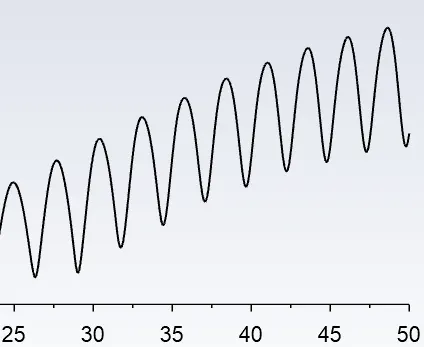
Fs = 10 / 25
Fs = 0.4
Charecteristic length L = 2m
Freestream velocity = 2.5m/s
Sr = (0.4 * 2 ) / 2.5
Sr = 0.8 / 2.5
Strouhal number = 0.32
Part 2 : Simulation for different values of Reynolds number
RE 10:
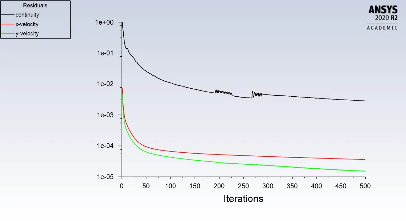
Residual plot:
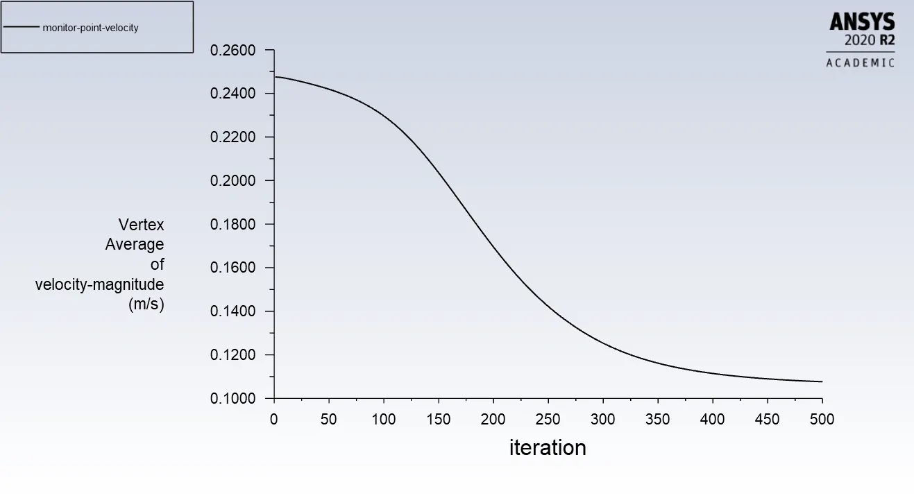
Monitor point velocity plot:
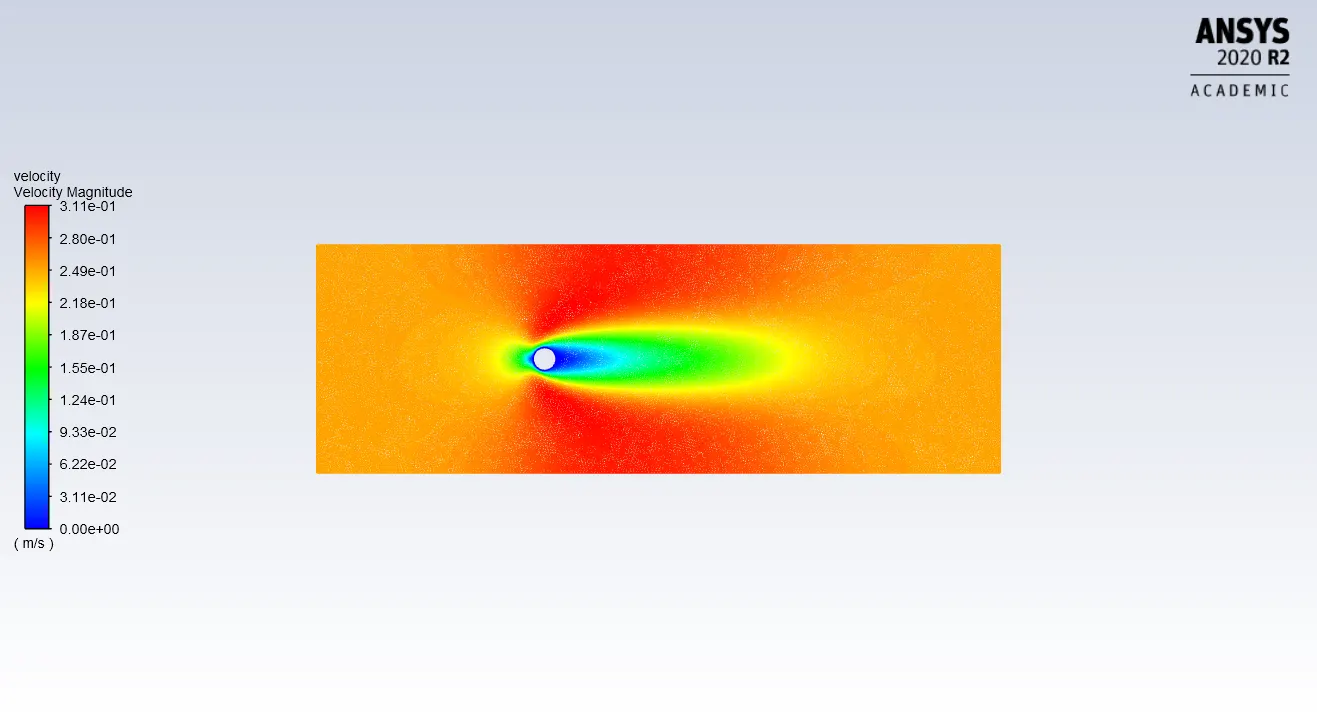
Velocity contour:
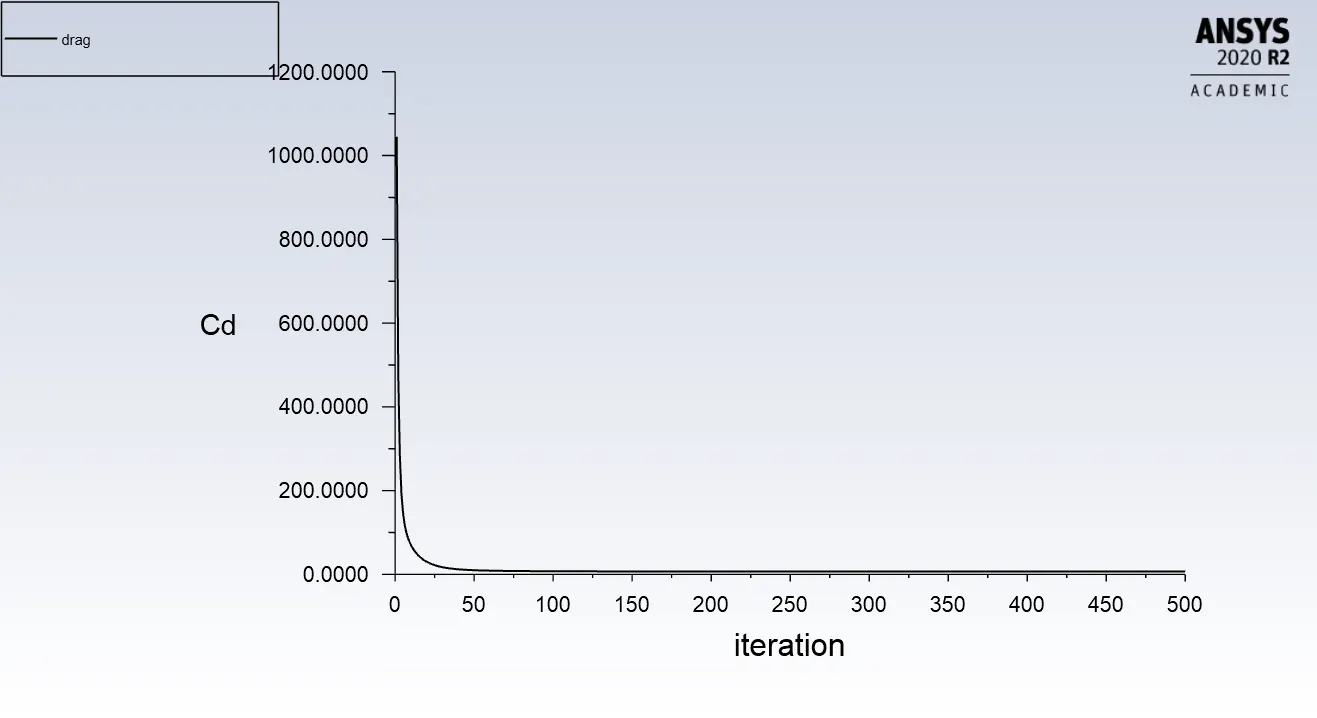
Drag coefficient plot :
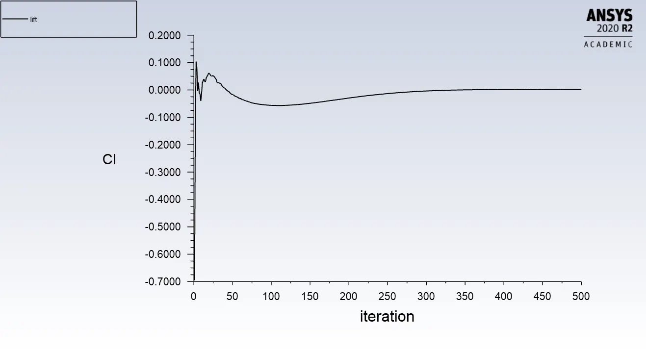
Lift coefficient plot:
RE 100
Residual plot:
Monitor point velocity plot:
Velocity contour:
Drag coefficient plot :
Lift coefficient plot:
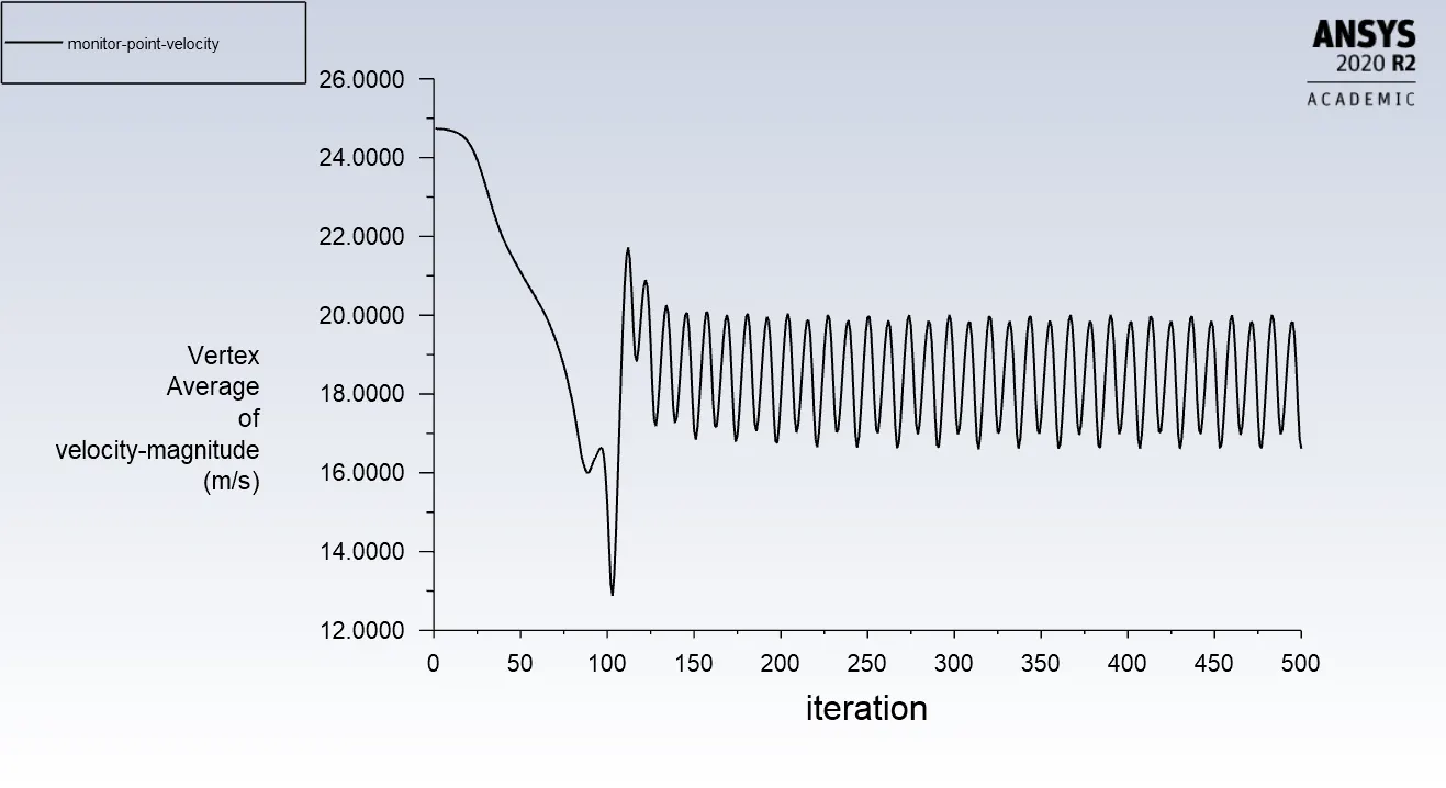
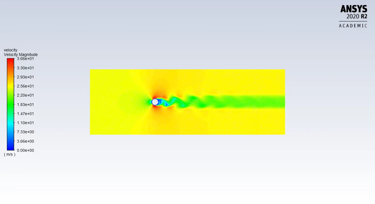
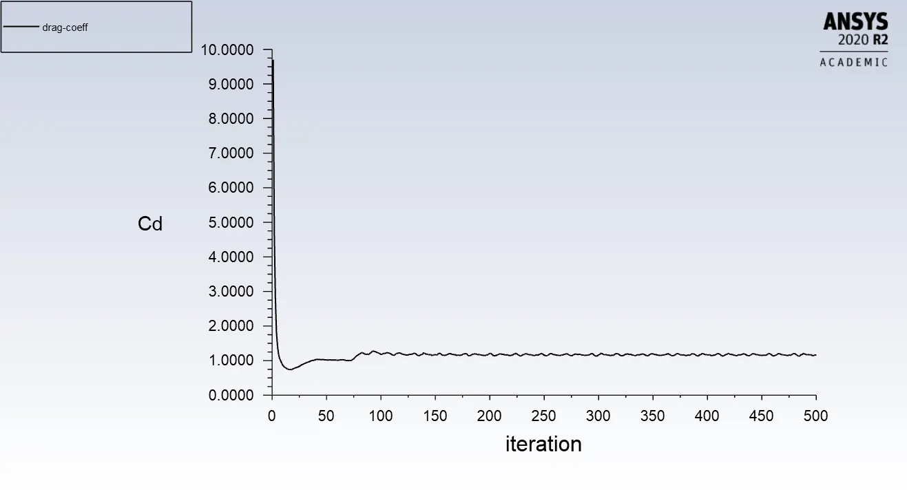
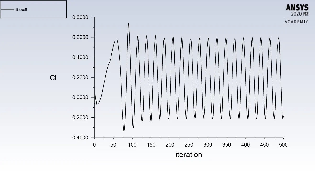
RE 1000
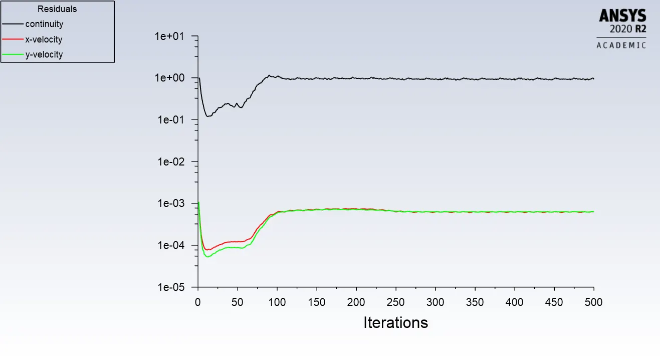
Residual plot:
Monitor point velocity plot:
Velocity contour:
Drag coefficient plot :
Lift coefficient plot:
RE 10000
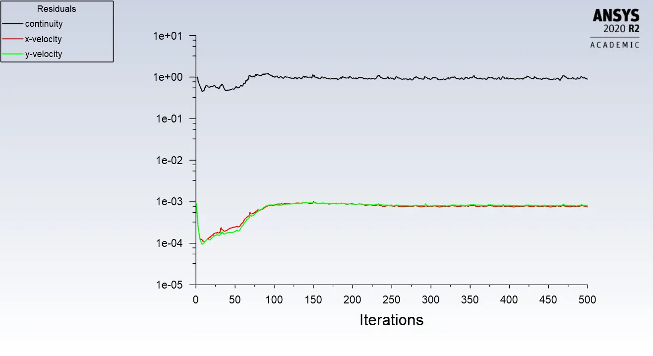
Residual plot:
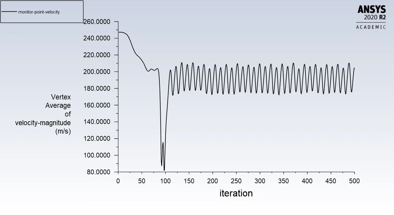
Monitor point velocity plot:
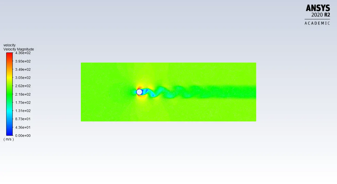
Velocity contour:
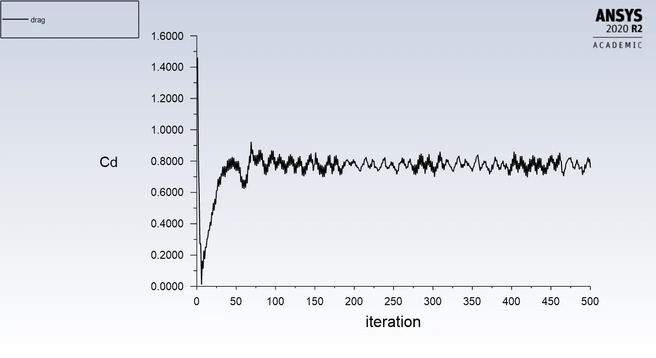
Drag coefficient plot :
Lift coefficient plot:
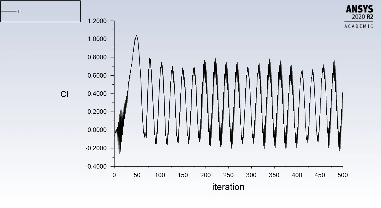
RE 100000
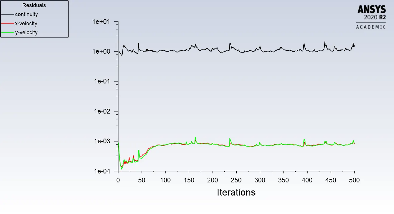
Residual plot:
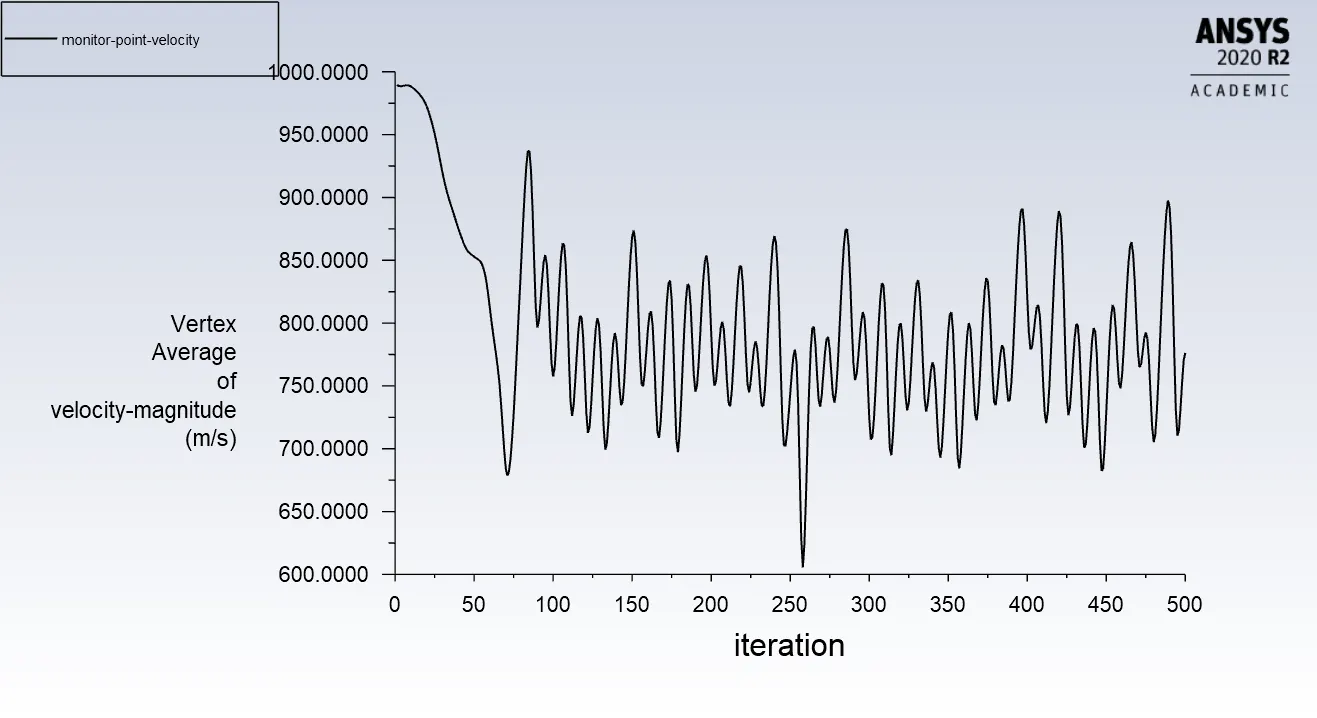
Monitor point velocity plot:
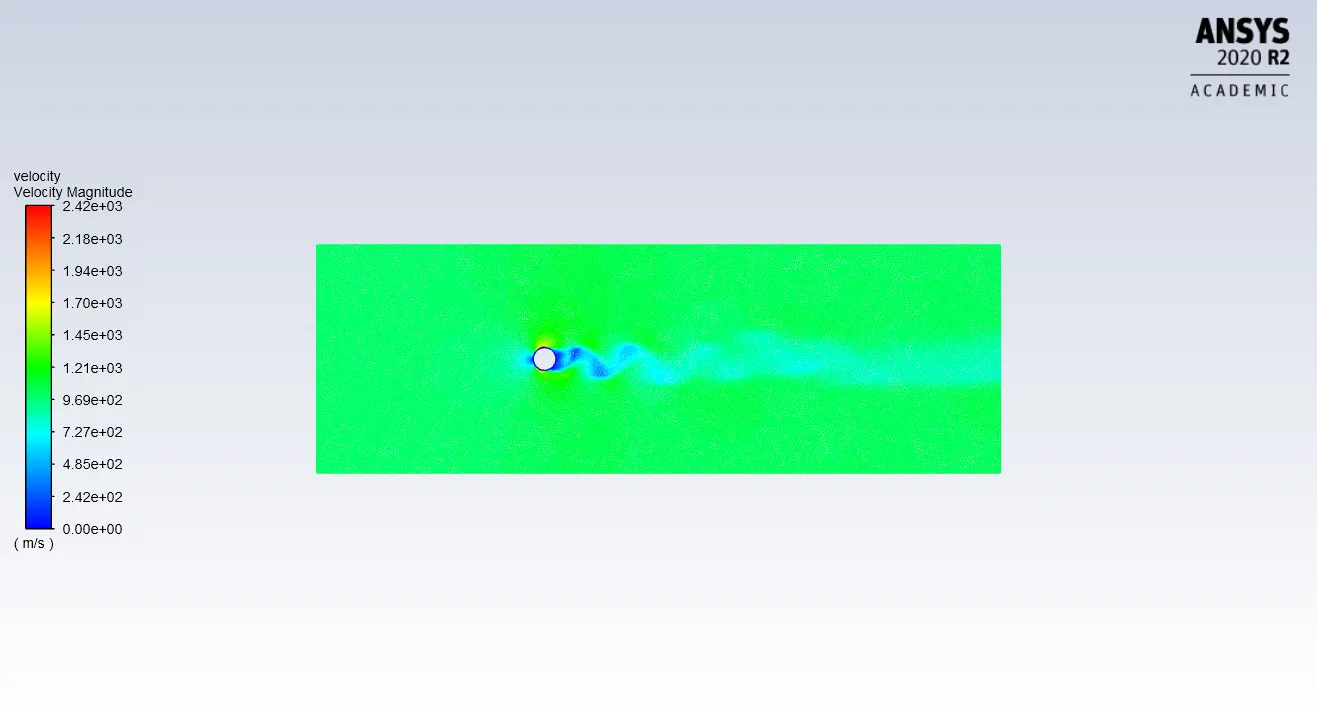
Velocity contour:
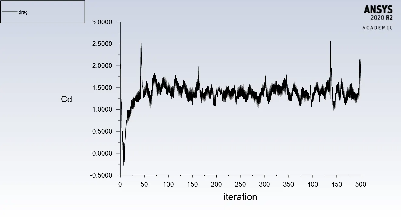
Drag coefficient plot :
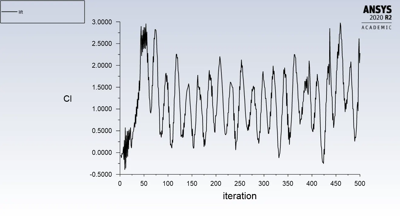
Lift coefficient plot:
Results and Conclusion :
> From the monitor point velocity plots and the velocity contours of the different cases seen above, it can be observed that all the cases except the one with reynolds number 10, Von Kármán vortex street is generated behind the cylinder.
> Convergence of the solution in each case can be verified by checking the plots of monitor velocity plots or coefficient of lift plots where it can be observed that the plots oscillates and this oscillation is stabilized over time.
The table below shows the setup and fluid propeties taken for diffrent cases:
| Length (m) | Density `(kg)/ m^3` | Viscosity kg/(m·s) | Velocity (m/s) | Reynolds number | Drag coefficient |
| 2 | 1 | 0.05 | 0.25 | 10 | 3.3287 |
| 2 | 1 | 0.05 | 2.5 | 100 | 1.3553 |
| 2 | 1 | 0.05 | 25 | 1000 | 1.2064 |
| 2 | 1 | 0.05 | 250 | 10000 | 0.9239 |
| 2 | 1 | 0.05 | 25000 | 100000 | 1.2212 |
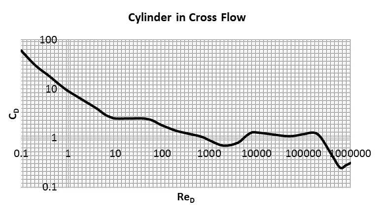
When the Re is less than 100 the drag coefficient is high and once it goes to and above 100 the drag coefficient can be seen reducing and has a small kink of increase at 100000 reynolds number.
The image below shows the plot of how the drag co efficient varies with resspect to variation in reynolds number and it can be observed that the values obtained from the simulation is not far off of experimental values.