Week 4 - CHT Analysis on Exhaust port

CONJUGATE HEAT TRANSFER ANALYSIS ON EXHAUST PORT

Aim:-

To perform a conjugate heat transfer analysis on the exhaust port to calculate the wall heat transfer coefficient on the internal solid surface and show the velocity and temperature contours plot.

Theory:-

1.Why CHT analysis is Used.

The Conjugate Heat Transfer (CHT) analysis type allows for the simulation of heat transfer between solid and fluid domains by exchanging thermal energy at the interfaces between them. A typical application of this analysis type exits as but is not limited to, the simulation of heat exchangers, cooling of electronic equipment, and general-purpose cooling and heating systems.

2. Where a CHT analysis is used.

The Conjugate heat transfer methods have become a more powerful tool for modeling and investigating the natural phenomena and engineering systems in different areas ranging from aerospace and nuclear reactors to thermal goods treatment and food processing, from complex procedures in medicine to atmosphere/ocean thermal interaction in meteorology, and from relatively simple units to multistage, nonlinear processes. A detailed review of more than 100 examples of conjugate modeling selected from a list of 200 early and modern publications shows that conjugate methods are now used extensively in a wide range of applications. The application in specific areas of conjugate heat transfer at periodic boundary conditions and in exchanger ducts is considered.

Y+ Calculation Formula:-

1. Reynolds number (Re).

`Re = (rho.U.D)/(mu)`

Where,

• Re = Reynolds number
• `rho` = Fluid density (`kg//m^3`)
• U = Free stream velocity (`m//s`)
• D = Diameter of the exhaust port (`m`)
• `mu` = Viscosity (`kg//m.s`)

2. Y+ value.

`y+ = (rho.U_(tau). Deltay)/mu => Deltay = (y+ . mu)/(rho.U_(tau)`

Where,

• `U_(tau)` = Frictional Velocity (`m//s`)
• `Deltay` = Absolute distance from the wall (or) Wall spacing (`m`)
• `rho` = Fluid density (`kg//m^3`)
• `mu` = Viscosity (`kg//m.s`)

3. Frictional Velocity (`U_tau`).

`U_tau = sqrt (( tau_w)/(rho))`

where,

• `tau_w`= Wall shear stress (`kg//m.s^2`)
• rho` = Fluid density (`kg//m^3`)

4. Wall Shear Stress (`tau_w`).

`tau_w = 1/2 . C_f.rho.U^2`

where,

• `C_f`= Skin friction coefficient
• rho` = Fluid density (`kg//m^3`)
• U = Free stream velocity (`m//s`)

5. Skin Friction Coefficient (`C_f`):-

`C_f = 0.079.Re^(-0.25)`

Simulation Process:-

1. Geometry (SpaceClaim).

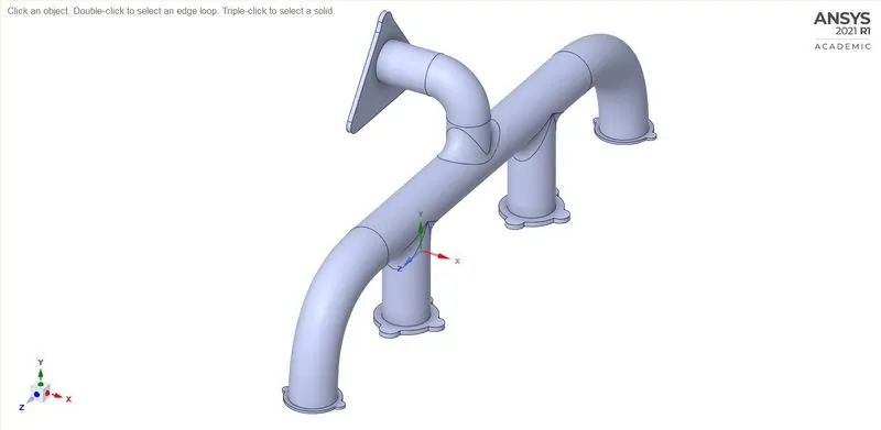
The exhaust manifold of 4 cylinder engine.

Volume Extraction:-

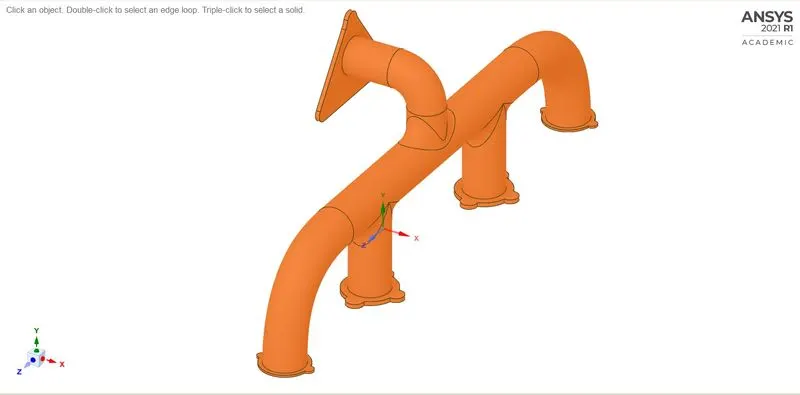
The Solid Volume.

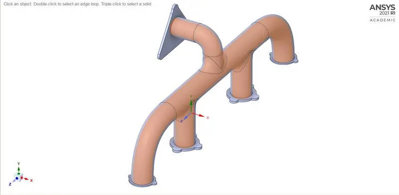
The Fluid Volume can be extracted by the "Volume Extraction" Command.

Share Topology:-

After the volume extraction, the fluid volume and solid volume should be shared. Shared topology is to achieve a conformal mesh where bodies meet, and the intersection of bodies has meshed perfectly. Shared topology is applied to volume and surface bodies that are completely inside the other volume or surface bodies.

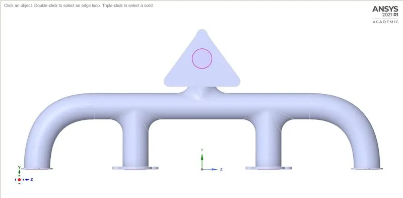
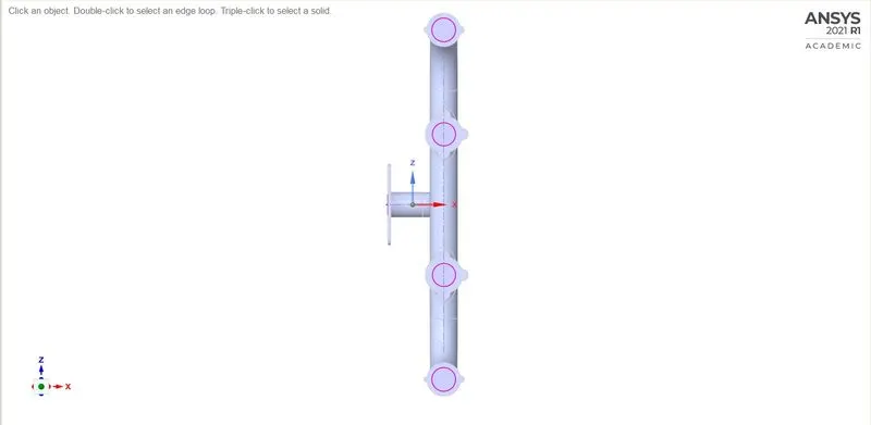
The 11 faces, 15 edges could be shared. After the completion of share topology, the fluid volume of the inlet and outlet is shown in a color.

2. Meshing.

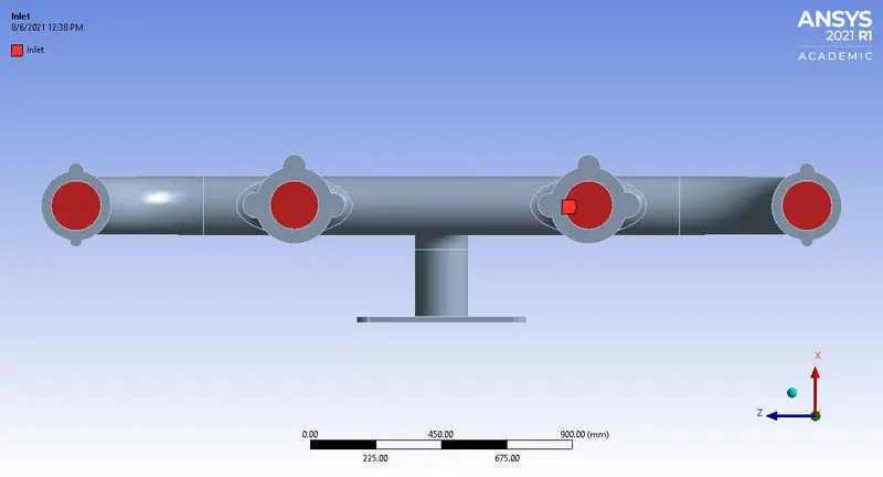
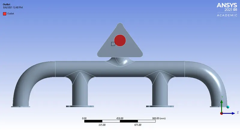
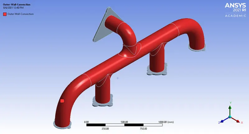
Named Selection:-

Inlet:-

Outlet:-

Outer-Wall-Convection:-

Inflation Layer:-

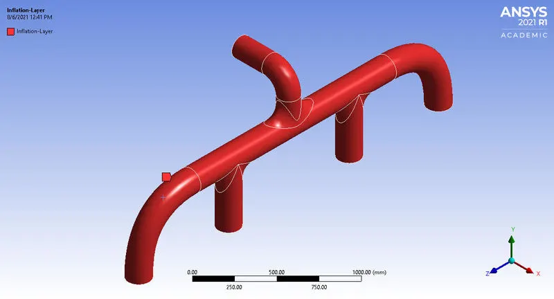
Compute the wall Spacing using the Y+ formula.

Required value:-

• Density (`rho`) = 1.225 `kg//m^3`
• Velocity (U) = 5 `m//s`
• Diameter (D) = 0.17 `m`
• Viscosity (`mu`) = 0.000017894 `kg//m.s`
• Y+ = 1

1. Reynolds number (Re).

`Re = (rho.U.D)/(mu)`

`Re = (1.225 xx 5 xx 0.17)/(0.000017894)`

`Re = 58189.89`

2. Skin Friction Coefficient (`C_f`).

`C_f = 0.079.Re^(-0.25)`

`C_f = 0.079 xx (58189.89)^-0.25`

`C_f = 0.005`

3. Wall Shear Stress (`tau_w`).

`tau_w = 1/2 . C_f.rho.U^2`

`tau_w = 1/2 xx 0.005 xx 1.225 xx 5^2`

`tau_u = 0.0765` `kg//m.s^2`

4. Frictional Velocity (`U_tau`).

`U_tau = sqrt (( tau_w)/(rho))`

`U_tau = sqrt((0.0765)/(1.225))`

`U_tau = 0.2499` `m//s`

5. Wall spacing (`Deltay`)

`Deltay = (y+ . mu)/(rho.U_(tau)`

`Deltay = (30 xx 0.000017894)/(1.225 xx 0.2499)`

`Deltay = 0.0017``m``=>` `1.7` `mm`

`therefore` Wall spacing = `1.7` `mm`

Compute the wall Spacing using the Y+ calculator.

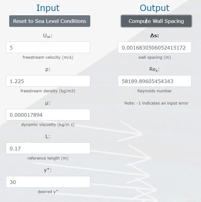
Wall Spacing = 0.00168 `m =>` 1.68 `mm`

From the both calculation the error is 0.02. so the First cell height is taken as a minimum value of 1.68 mm.

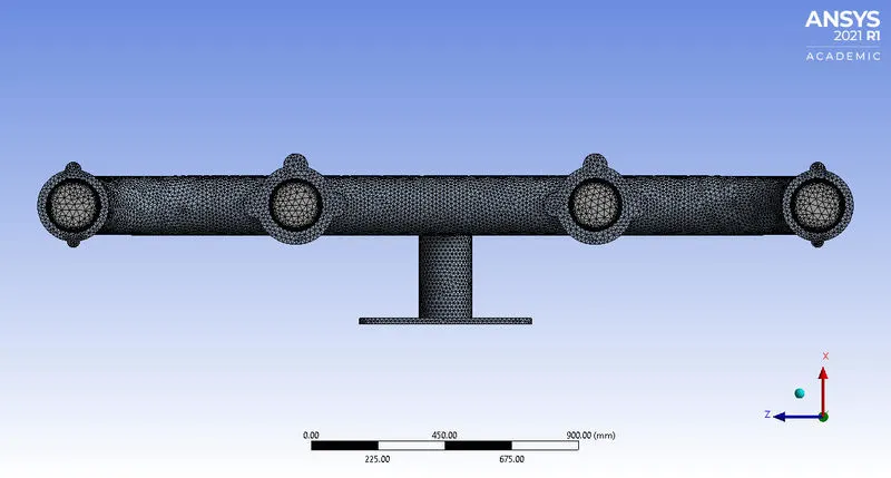
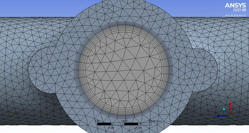
Calculate Total Thickness for Inflation Layer:-

Layer No	Layer Thickness (mm)	Growth Rate
1	1.68	20% (1.2)
2	2.02
3	2.42
4	2.90
5	3.48
Total Thickness	12.5

After calculating the Total thickness applied in Fluent Meshing.

Body Sizing:-

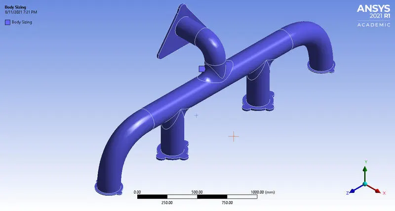
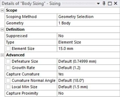
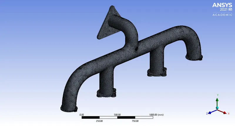
• Element Size = 15 mm
• Capture curvature = yes

Mesh:-

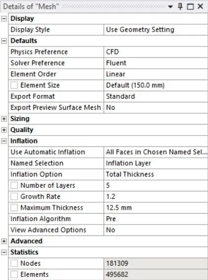
• Y+ = 30
• First Cell Height = 1.68 mm
• Maximum thickness = 12.5 mm
• Number of layers = 5
• Growth rate = 1.2
• Elements = 495682

Inflation Layer:-

3. Setup & solution (Fluent).

• Solver = Pressure based Solver
• Time = Steady
• Energy Equation = Enable
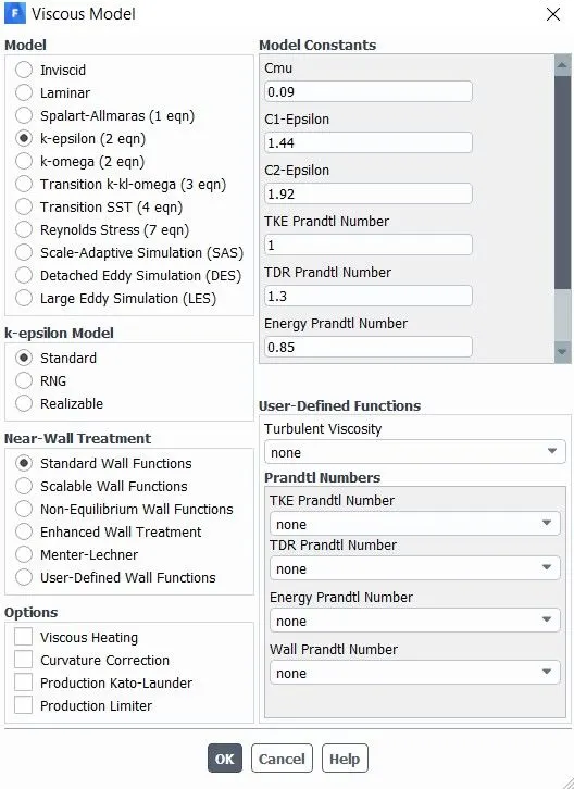
• Viscous model = k-epsilon

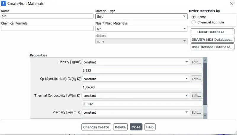
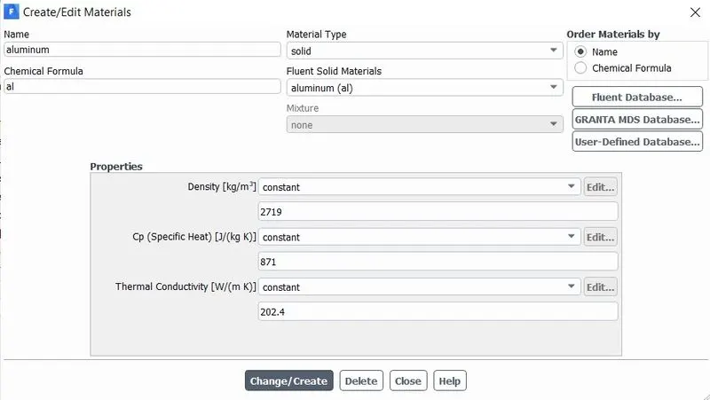
• Material = Fluid volume is air, Solid volume is aluminum

• Boundary condition

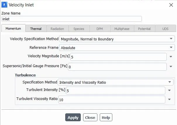
1. Inlet = velocity 5m/s, Temperature = 700 K.

2. Outlet = 0 (Gauge pressure)

3. Wall convection = Thermal condition-convection, Heat transfer coefficient = 20 W/(m^2.K)

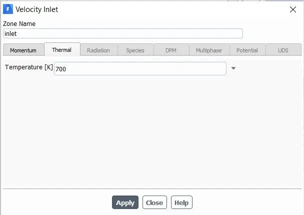
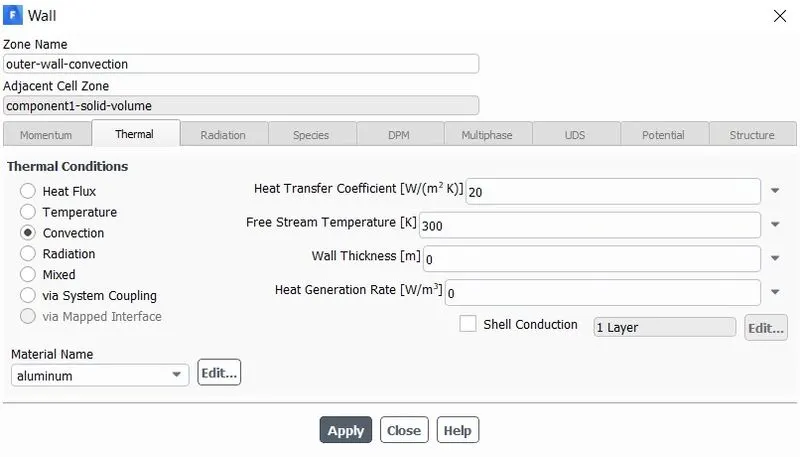
• Initialize with Hybrid method solution.
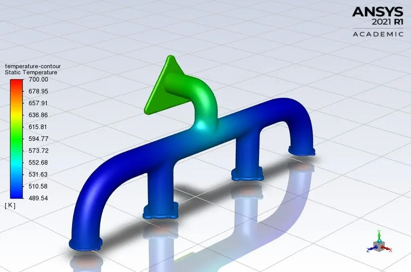
• reate Temperature contour to visualize the changes.
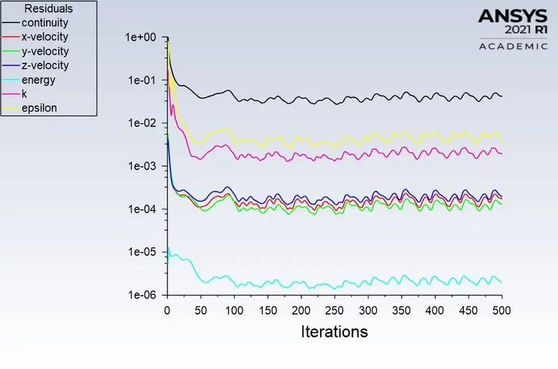
• Run for 500 Iterations.

Contour of static Temperature.

Residuals.

4. Post-Processing Result.

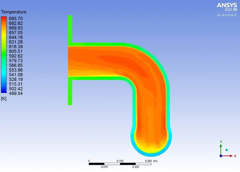
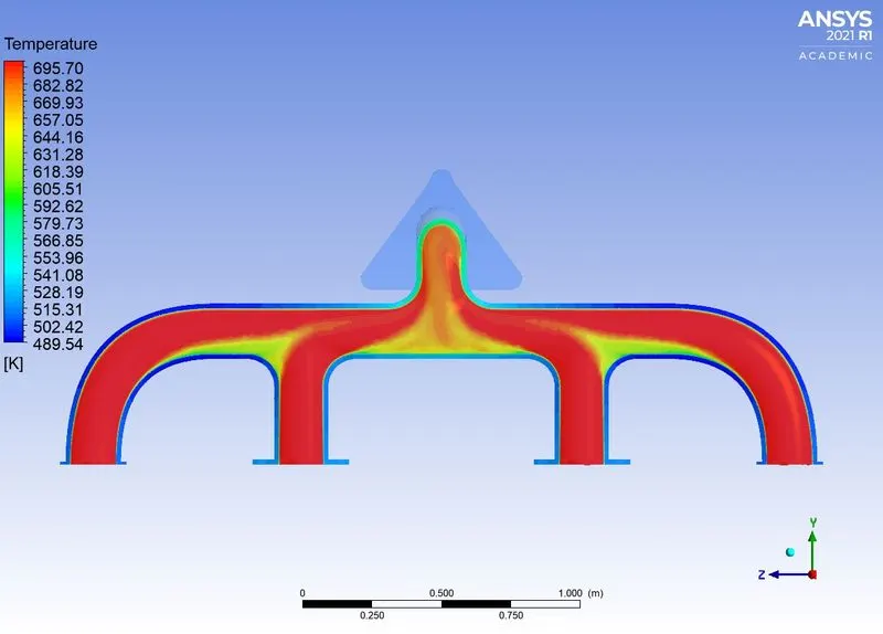
1. Temperature:-

2. Velocity Contour:-

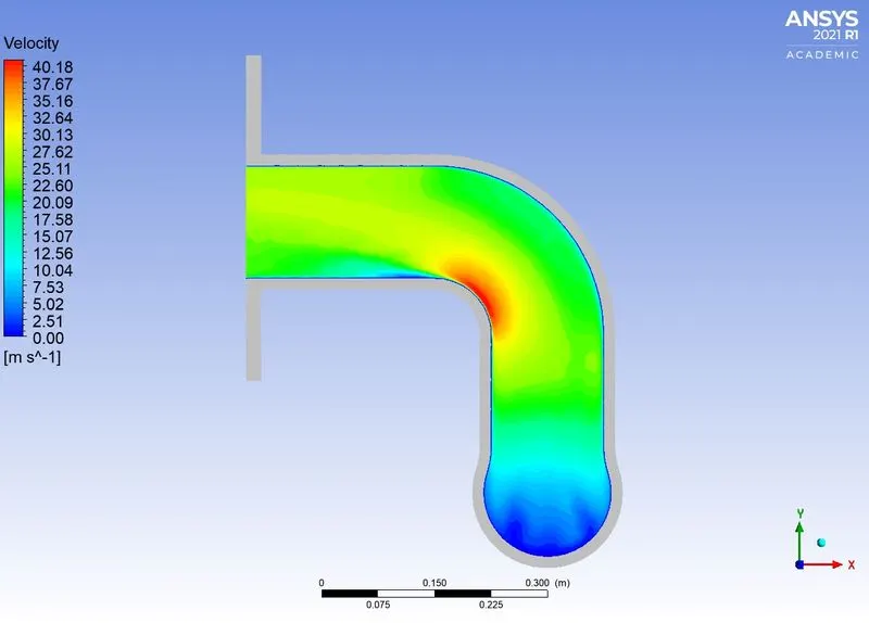
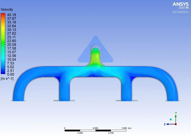
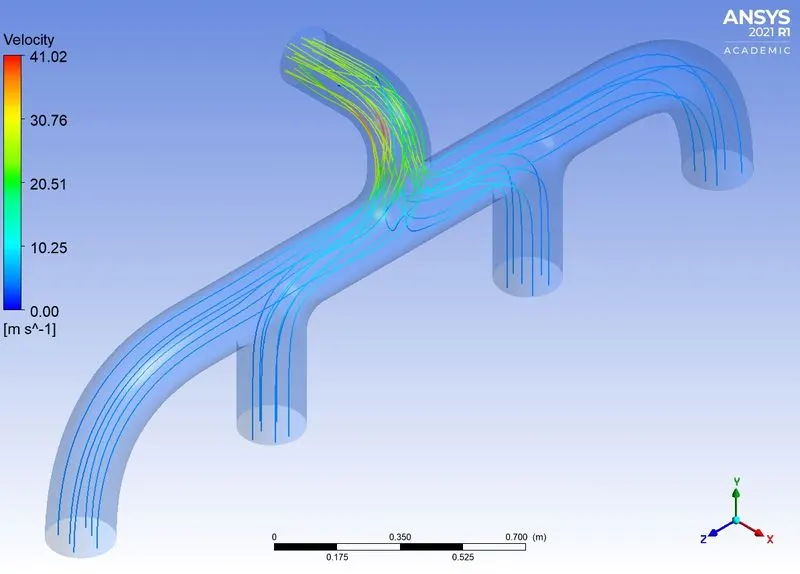
In a velocity contour the velocity is maximum the outlet area. Because, the exhaust gas of four inlet area should be flow in a single outlet area. At the bend of the exhaust pipe region, the velocity is higher than the other region.

3.Velocity streamline:-

4. Wall Heat Transfer Coefficient:-

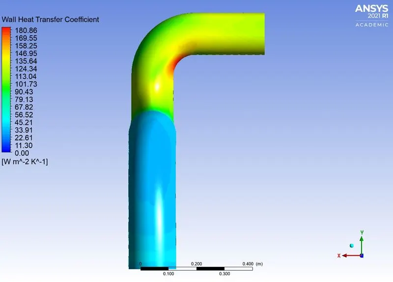
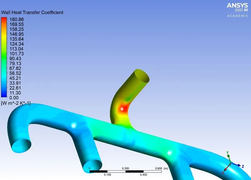
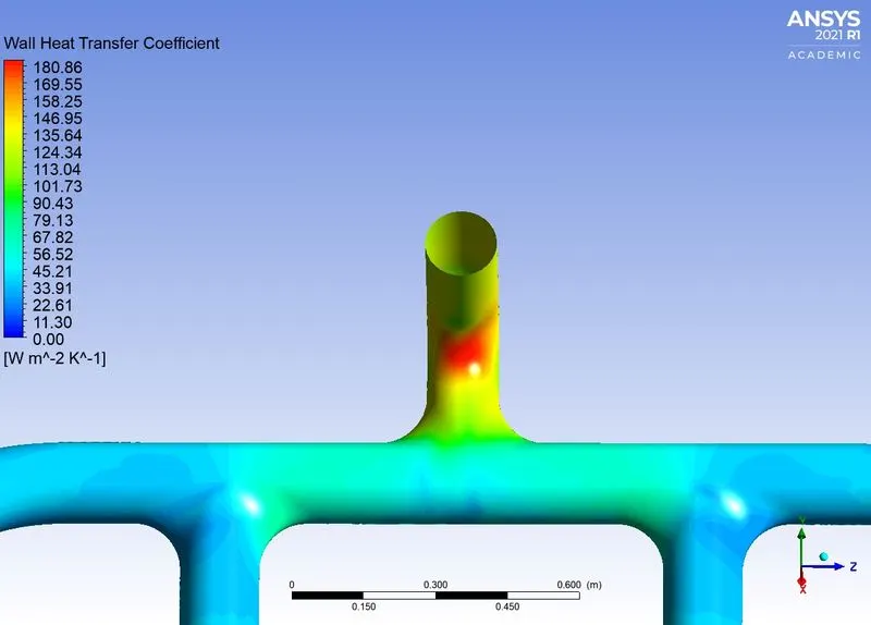
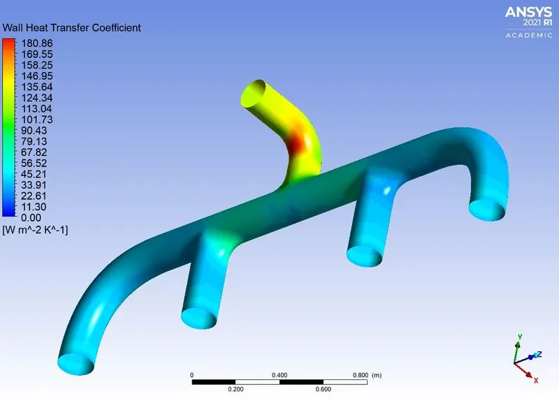
In the plot, the wall heat transfer is higher in the exhaust pipe bent region due to the higher velocity.

Heat Transfer Coefficient is = 180.86 `W//m^2.K`

How Would you verify if the HTC prediction from the simulation are right? On what factor does the accuracy of the prediction depend on.

Nusselts Number :-

`Nu = (h.L)/K` `=> h = (Nu.K)/L`

where,

Nu = Nusselt's Number.

h = Heat Transfer coefficient.

K = Thermal conductivity.

L = Charecteristic Length.

The Nusselt's number is a function of reynolds number, which in turn is a function of flow velocity. Therefore, HTC is directly proportional to flow velocity.

From the Heat transfer coefficient and velocity plot are maximum near the outlet region.

Factors does the accuracy depends on.

• Selection of Turbulence model based on the y+ value.
• Inflation layer increase the Mesh quality in the boundary region help to capture the accurate result.
• The Fluid and solid interface should be in conformal mesh.

Conclusion:-

• The velocity is increase from the inlet to the outlet because of mass conservation.
• The wall Heat transfer Coefficient is high at the bend junction due to the high velocity of the exhaust gas and when the heat is transferred from fluid to solid the HTC is also high.
• The Reynolds number and wall spacing is calculated from the formula and the Y+ calculator is same, so that the turbulence model is correct according to the Y+ value.