CHT Analysis on Exhaust port
OBJECTIVE
- To perform Conjugate Heat Transfer (CHT) simulation on an exhaust export.
- To study and understand where and why CHT analysis is conducted.
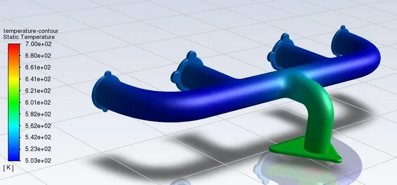
- To plot appropriate wall/surface shear stress, velocity, and temperature contours.
Conjugate Heat Transfer (CHT):
- It basically tells about the simulation of a combination of heat transfer between solid and fluid domains with the thermal energy exchange at their interfaces.
- It provides effective heat transfer by combining efficiently the heat transfer between solid and fluid which is instrumental in the designing of coolers, heaters, and heat exchangers.
- Designing energy-efficient devices by minimizing unwanted heat losses.
- They are used in some applications like aerospace (for example, analysis of gas turbine engines to improve efficiency), electronic circuit board (for example, improve heat transfer in the heat sink so as to provide sufficient cooling in the microprocessor), pumps & compressors, after-treatment systems (for example, predicting urea deposition in the vulnerable areas of the wall by analyzing the wall temperature, electromobilities, etc.
Steps:
- This simulation is basically performed to understand the idea of conjugate heat transfer between solid and fluid. We have taken the exhaust port model here to do the analysis.
- The fluid volume inside the model is created using the volume extract tool.
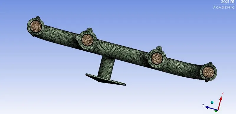
- Share tool under Workbench is used and Share topology is set to share to seamlessly carry out the communication between the solid and fluid volumes during meshing.
- Different mesh sizes are used in each case. The body (outer wall of solid volume) sizing size is also refined in respective cases.
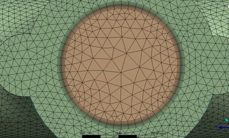
- the y+ value is maintained and depending on the same, inflation layers are given to precisely capture the near-wall treatment.
- For solving, we use steady-state and pressure-based solvers.
- The turbulence model used is K-epsilon with Standard wall function.
- The initial condition for velocity inlet is 5 m/s in one case and 10 m/s in another and for temperature, it is 700 K. The outer surface wall convective heat transfer coefficient is given 20 W/m²K.
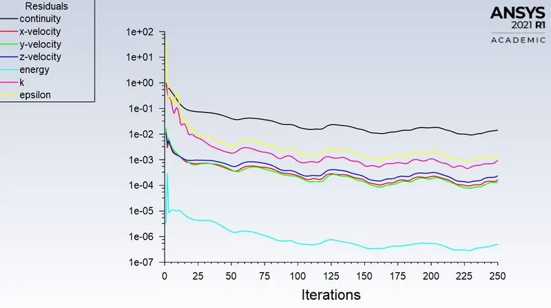
- We run the simulation until converged and the desired results are calculated.
Mesh:
Inflation layers:
- Case 1
Mesh size = 100 mm
Body (solid surface) sizing = 20 mm
Velocity of fluid at inlet = 5 m/s
Convergence Plot:
Temperature Contour:
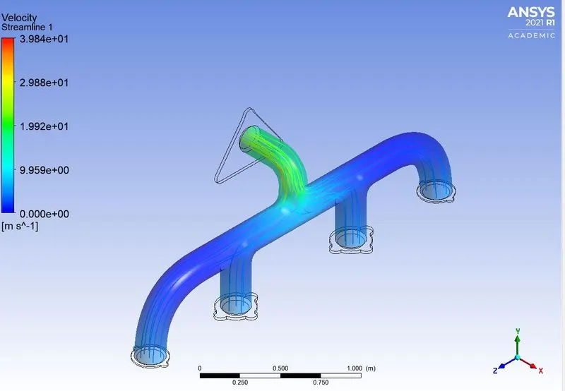
Streamline (velocity) Plot:
Wall Heat Transfer Coefficient Plot:
- Case 2
Mesh size = 100 mm
Body (solid surface) sizing = 40 mm
Velocity of fluid at inlet = 5 m/s
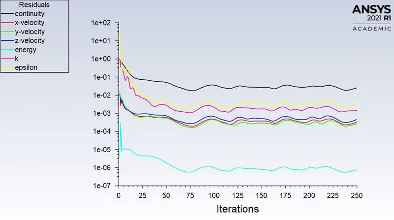
Convergence Plot:
Temperature Contour:
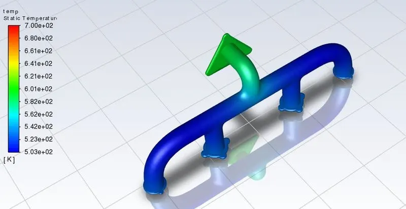
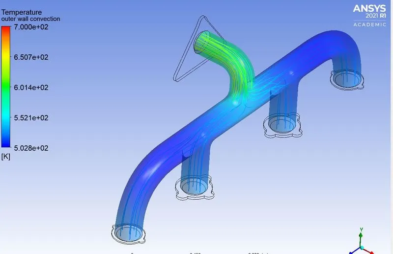
Streamline (velocity) Plot:
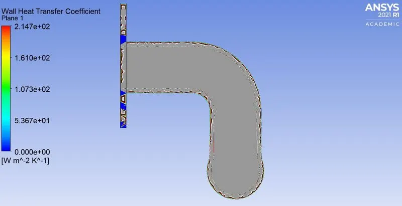
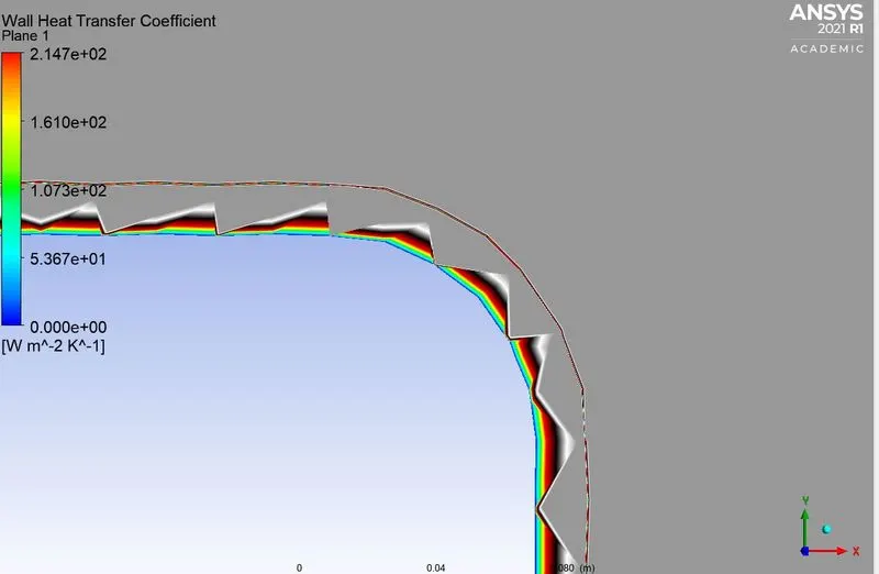
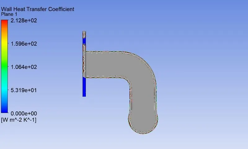
Wall Heat Transfer Coefficient Plot:
- Case 3
Mesh size = 100 mm
Body (solid surface) sizing = 40 mm
Velocity of fluid at inlet = 10 m/s
Convergence Plot:
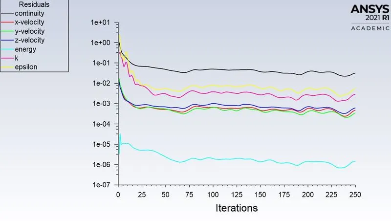
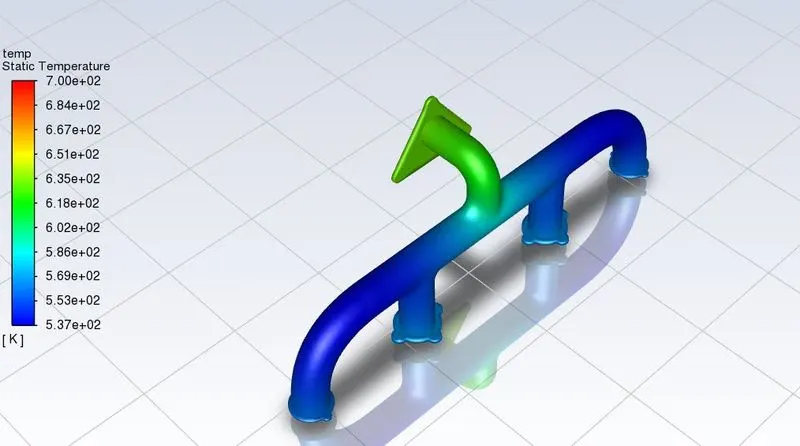
Temperature Contour:
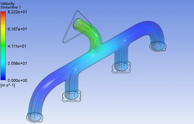
Streamline (velocity) Plot:
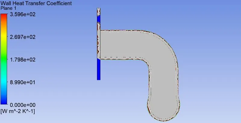
Wall Heat Transfer Coefficient Plot:
Inference:
The simulations have been conducted for three cases. The cases include refined mesh conditions and case where the velocity is different. It has been observed that when the mesh is refined precise and improved results are captured. The wall heat transfer coefficient is found to be maximum at the outlet region as shown in the HTC plot. In the velocity streamline plot, it can be noted that the velocity at the same place is found to be maximum. This is because of mass conservation. All the volumetric flow rate through the inlets simultaneously exits through the outlet resulting in the increased velocity at the outllet. When the velocity increases corresponding wall heat transfer also increases. The value of HTC is found to be increasing in the case when velcoity value at the inlet is given more than the initial cases.