CHT Analysis on Exhaust port

AIM:

To perform a CHT analysis on a exhaust manifold

INTRODUCTION:

The analysis type of Conjugate Heat Transfer allows the simulation of the heat transfer between solid and fluid domains by exchanging thermal energy at the interface between them. Typical applications of this analysis type are the simulation of the heat exchanger, cooling of electronic equipment, and general-purpose cooling and heating system. In most cases, heat transfer in solids, if only due to conduction, is described by Fourier's law of heat conduction.

In most cases, heat transfer in fluids, if only due to convection, is described by Newton's law of cooling. The Conjugate Heat transfer corresponds with the combination of heat transfer in solids and heat transfer in fluids. Conjugate Heat Transfer Applications: 1) Heat exchanger - It exchanges heat from one fluid to another. The forced convection is the most common way to achieve a high heat transfer coefficient. The separation layers are made of solid. The conduction occurs through the separation layer.

2) Thermal insulators (eg. Polyurethane foam) - Polyurethane foam contains cavities of air which gives the insulation property to the material.

3) Heat sink - It dissipates the heat from electronic devices through convection. 4) Exhaust port manifold- It transfers the burned air mixture from all cylinders to exhaust system. the solid part of manifold takes heat from hot gas through convection. then the heat is conducted through the solid part of the manifold. Finally, the heat dissipated through the outer surface of the manifold.

PROCEDURE:

1.Open Ansys Workbench and import Ansys Fluent module into it

2. Next we import the geometry into geometry section. The below shown image is teh geometry

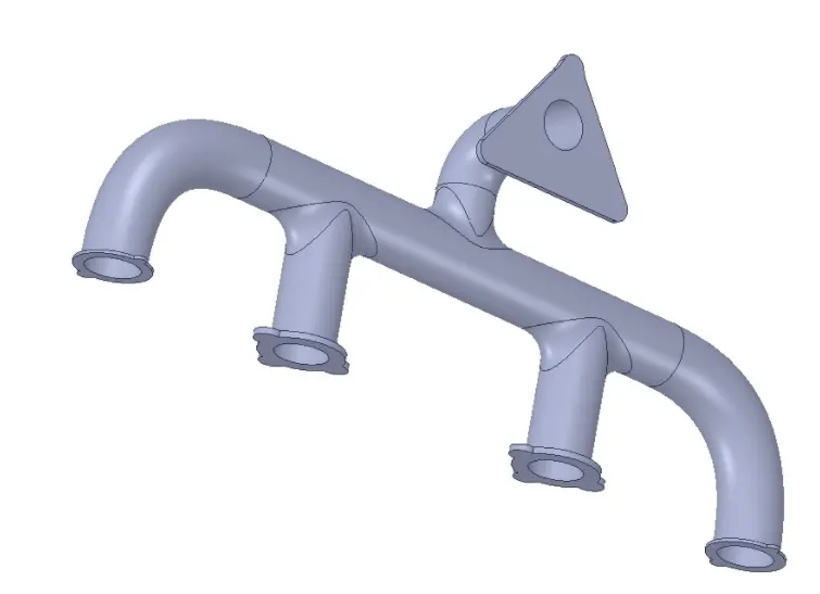
FIG 1: Exhaust port manifold for 4 cylinders in-line engine

3. As we are done with geometry setup next task is to mesh the model which is done in the mechanical module

4.The Academic version of Ansys has an element count limit of 0.5 million. Hence, the maximum number of elements have been limited to 0.35 million.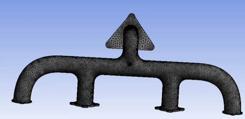

FIG 2:MESHED MODEL
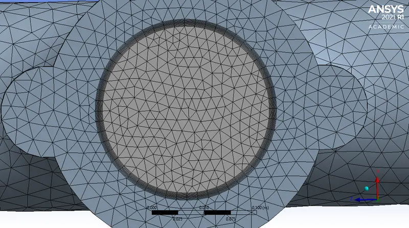
5.Here a y+ value of 5 is assumed which falls in the range of k-omega which is best suitable turbulence model for this exhaust port simulation

6

FIG 3: 6 Inflation Layers added

6.The above pictures show that the mesh details of inflation layers, Fluid and solid domain which helps to capture the wall effects

7.Nextlywe have to add the name selected for easiness in applying the boundary conditions

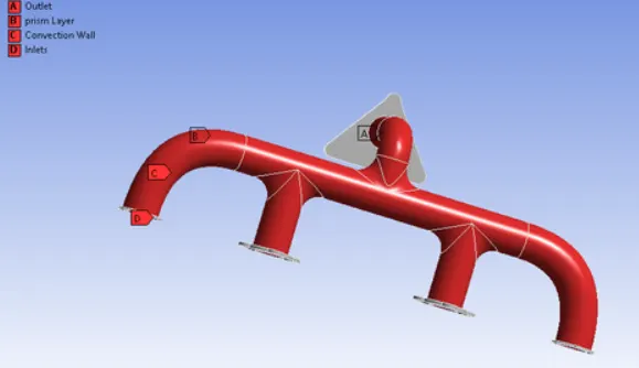
8. Now as we are done with meshing and named selection we move onto setup for setting up the simulation

SIMULATION DETAILS

Type of simulation: Steady-state

Type of model: K-omega (Turbulence model)

Material Properties:

The material of Exhaust manifold: Aluminum

Working fluid: Air:

Density = 1.225 `(Kg)/(m^3)`

Specific heat `c_p`=1006.43 `J/(Kg*K)`

Thermal conductivity = 0.0242 `W/(m*K)`

Viscosity = 1.7894e-5 `(Kg)/(m*s)` Aluminum: Density = 2719 `(Kg)/(m^3)`

Specific heat `c_p` = 871 `J/(Kg*K)`

Thermal conductivity = 202.4 `W/(m*K)`

Boundary condition:

Inlet air velocity = 5 m/s

Inlet air temperature = 700 K

Outlet pressure = 0 Pa

The outer surface of Exhaust manifold: Wall

Thermal condition = Convection

Heat transfer coefficient = 20 `W/(m^2*K)`

Solution method: Pressure-Velocity coupling

9. Now as the simulation parameters are set up we move onto the result part. The solution is run for 300 iterations and results can be viewed below

RESULTS:

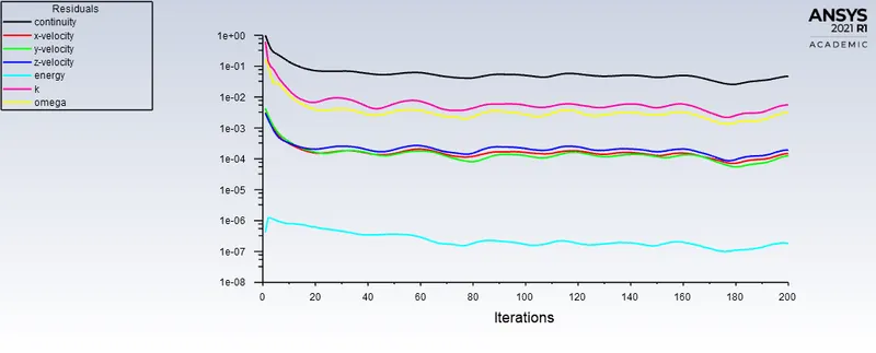
FIG 4:RESIDUAL PLOT OF REFINED MESH CASE

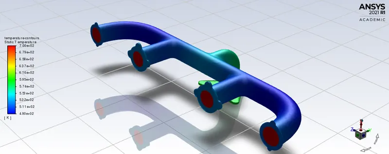
FIG 5:TEMPERATURE CONTOUR

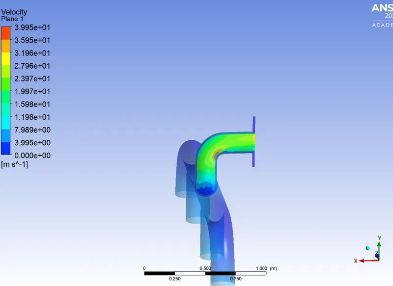
FIG 6:VELOCITY CONTOUR

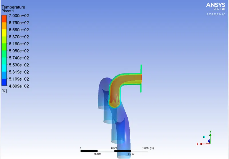
FIG 7 :TEMPERATURE CONTOUR

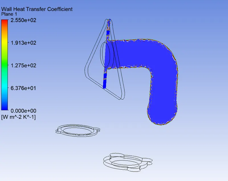
FIG 8:WALL HEAT TRANSFER COEFFICIENT

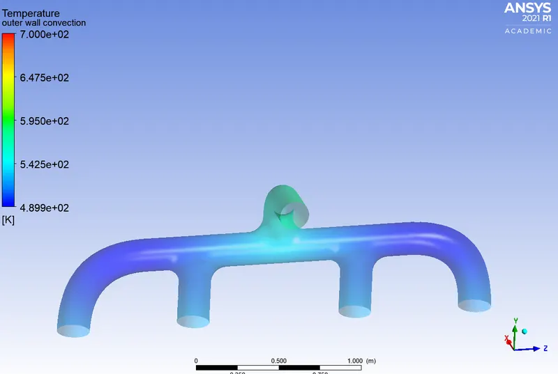
FIG 9:INLET TEMPERATURE CONTOUR

3) How would you verify if the HTC predictions from the simulations are right? On what factors does the accuracy of the prediction depend on?

1. Nusselt number

Nusselt's number is given by:-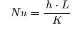
where. h= Heat Transfer Coefficient

Nu= Nusselt's Number

K= Thermal conductivity coefficient

L= Characteristic Length

We know that Nusselt's number is a function of Reynold's number, which in turn is a function of flow velocity . Therefore, HTC is directly proportional to flow velocity. Calculating theoretically:

R = (Convection resistance) Out + Wall Conductivity resistance + (Convection Resistance);

R = `1/(hout)+L/K+1/(hin)`

R= `1/20+0.015/202+ 1/(hin)`
Here, at node point: q = 6987.5 W/m2K, Bulk Temperature = 682.31 K
Therefore,
After substitution we get,
AT= 682.31 — 300 = 381.31 K
hi„ = 215.55 W/m2K

2) Grid dependence test Conclusions: 1) The results obtained from baseline mesh and refined mesh followed the same pattern of contour. But the magnitude of the temperature and velocity are slightly varied. 2) The simulation results obtained from simulation were verified using the Dittus-Boelter equation. 3) The accuracy of the prediction depends on mesh quality, Number of elements, usage of Inflation layers.

CONCLUSION
• The velocity tends to increase from the inlet to the outlet because of mass conservation and the mixing of air. hence, the high heat transfer coefficient at the junction is due to that high velocity and also when the transfer of heat from the fluid to solid is high.

• The internal flow velocity and its characteristics are affected by the Initial velocity, Pressure, the physical features of the geometry etc. that affect the heat transfer rates, and hence CHT analysis is essential prior to experimental analysis for better prediction life of the designed component.

• As shown in the plots, the hot exhaust gases passing through the manifold transfer some of the heat to it via convection. The amount of heat transfer can be related directly with the velocity of the exhaust. The temperature is lower where the flow is stagnating or is moving at the inlet velocity. As the velocity increases, so does the Reynolds number and hence the amount of heat transferred.

• Best method to predict the accuracy of the result is by comparing the nusselt numbers from experiments and numerical results. The other method to verify is by comparing the results from published experimental results.