Week 4 - CHT Analysis on Exhaust port

AIM: To simulate conjugate heat transfer through of an automobile exhaust port.

OBJECTIVE:

1. Observe the y+ value over the geometry.

2. Create an animation of parameters varying through the geometry.

3. Calculate the wall/surface heat transfer coefficient on the internal solid surface & plot the velocity & temperature contours.

THEORY AND EXPLANATION:

Conjugate heat transfer: Conjugate heat transfer corresponds with the combination of heat transfer in solids and heat transfer in fluids. In solids,
conduction often dominates whereas, in fluids, convection usually dominates. Conjugate heat transfer is observed in many situations. For example, heat sinks are optimized to combine heat transfer by conduction in the heat sink with the convection in the surrounding fluid.

Applications:

• HVAC
• Heat Exchanger
• Tank
• Internal Combustion Engine
• Heat Sink
• Boiler
• Reactor
• Heat Pipe
• Turbocharger

PROCEDURE:

The given model was imported to space claim and the model was checked for duplicate edges using the extra edges tool. The required fluid volume was extracted using the extract volume tool.

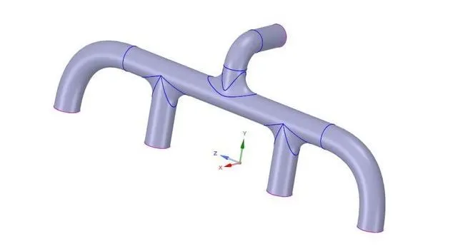
The solid and fluid volume components are selected and moved to a new component and named final geometry and Shared topology is enabled.

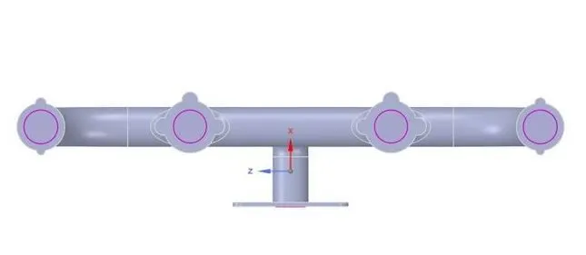
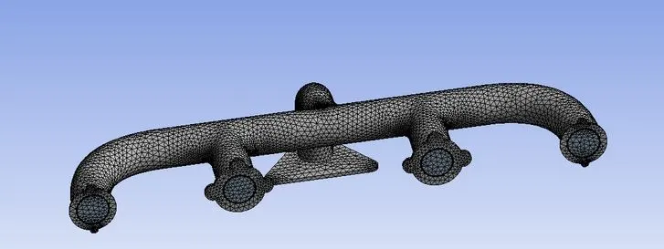
Since it is a baseline simulation, the default meshing that Ansys mesher does is checked. Named selections are provided to all
the parts to apply boundary conditions when physics is set up. There are three named selections

1. inlets, from where the hot exhaust gases enter the exhaust manifold

2. outlet, from where the exhaust gases leave

3. outer wall convection

CASE SETUP:

• In the setup, we are setting up the physics of the simulation.
• Setup>physics>general setting>solver>type>pressure based.
• Setup>physics>general setting>time>steady.
• physics>model>check energy.
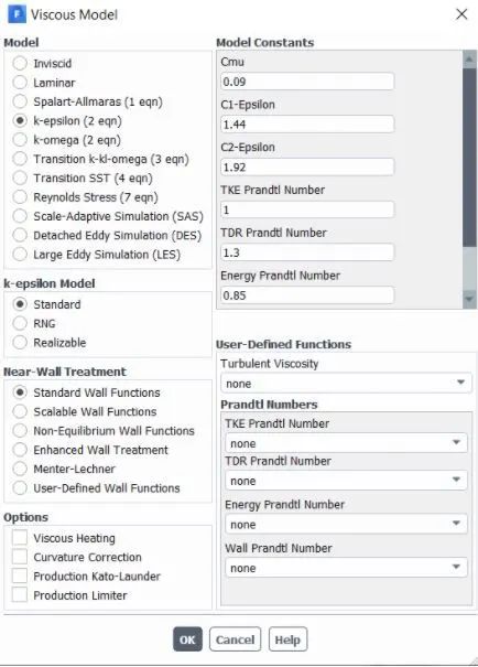
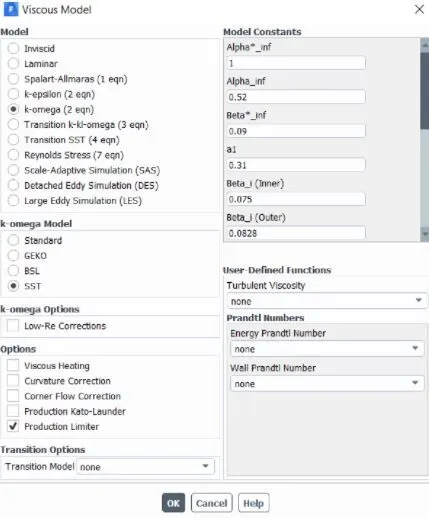
• physics>model>viscous model>K-epsilon or K-Omega, in the baseline I have taken the K-epsilon model and for refined mesh, i have taken K-Omega, SST model.
• physics> material>material type>fluid/solid.
• physics> material>fluent fluid material>air/aluminium.
• physics> material>properties> I have taken the default values here.
• physics>zones>boundaries>inlet> velocity as 5m/s and in thermal properties temperature as 700k and rest of all are default values.
• physics>zones>boundaries>outlet>gauge pressure as 0.
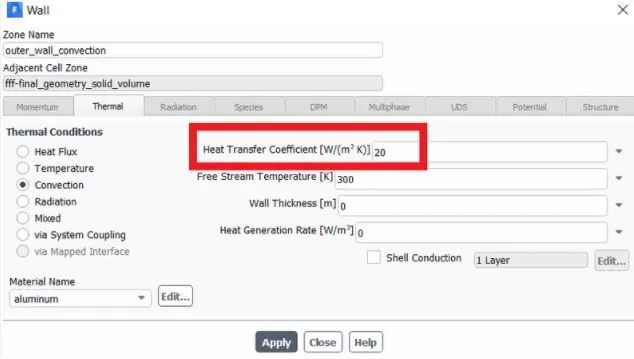
• physics>zones>boundaries>outer convection wall>thermal>convection, HTC as 20 w/m^2k, free stream temperature as 300k.
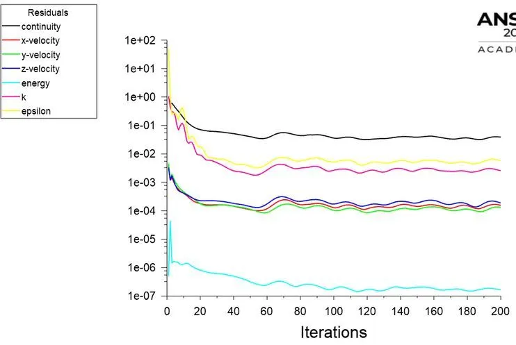
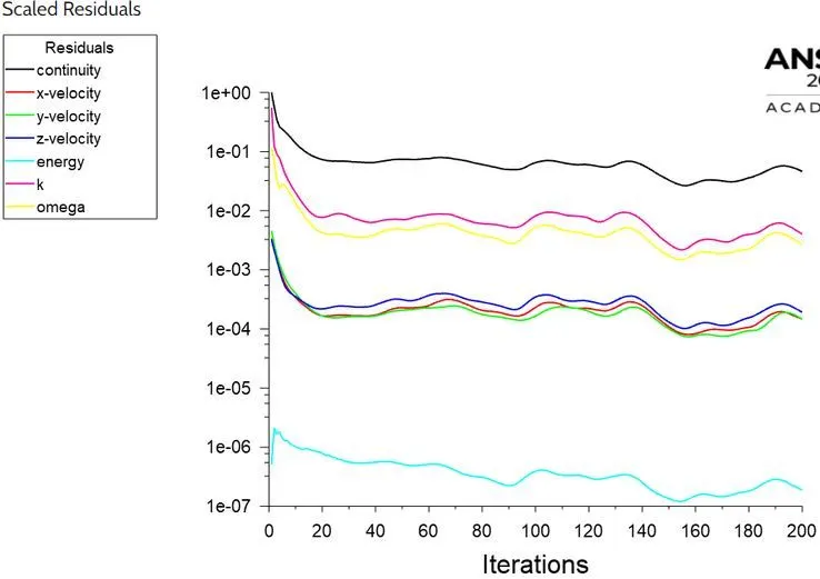
• Setup>solution>report>residuals>uncheck all the absolute convergence criteria and using the hybrid method initialize the simulation and run the simulation for the required number of iterations.

RESULTS:

CASE1: K-EPSILON SOLVER

SCALED RESIDUALS:

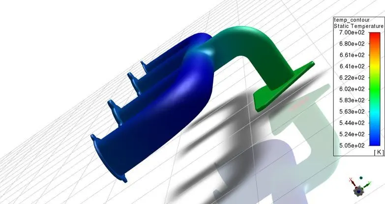
TEMPERATURE CONTOUR:

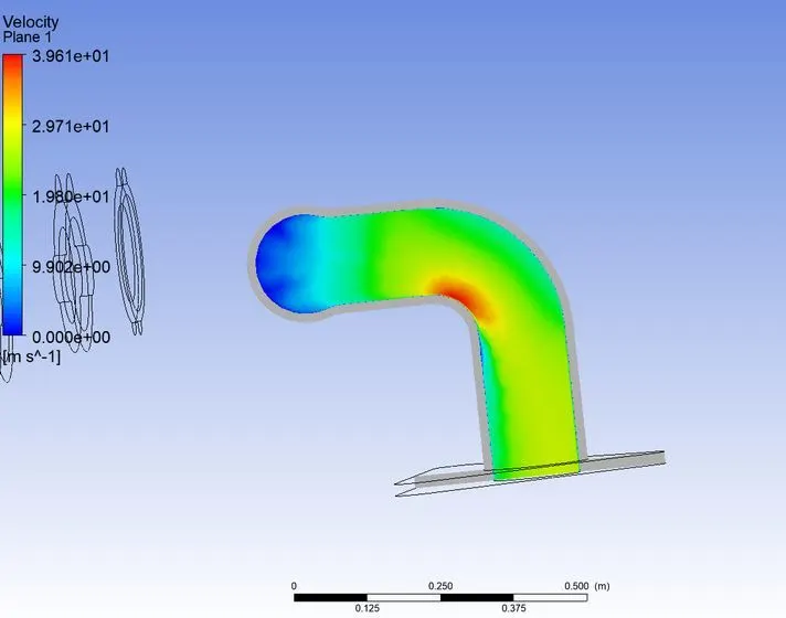
VELOCITY PLANE:

CASE2: K-OMEGA SOLVER

SCALED RESIDUALS:

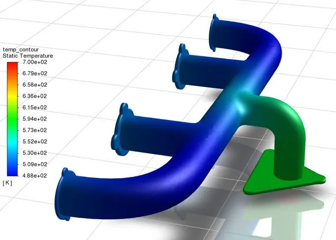
TEMPERATURE CONTOUR:

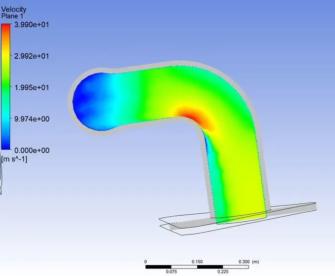
VELOCITY PLANE:

CONCLUSION:

1. As the temperature of the pipe at the outlet has increased. This is because at the outlet all the inlets converge, therefore to conserve the mass velocity has increased. Due to the increase in velocity heat transfer due to convection has increased.

2. There is no change in temperature difference in all the cases but the change in minimum temperature.

3. The velocity and hence the Reynolds number is higher at the outlet. Due to that, the heat transfer and temperature is higher.

4. The heat transfer coefficient is higher between fluid and solid at the outlet pipe, because the velocity of the fluid is higher