CHT Analysis on Exhaust port

Aim:

To run a simulation to analyze Conjugate Heat transfer in Exhaust port.

Objective:

1. To understand why and where a CHT analysis is used.
2. To perform a CHT analysis on exhaust port manifold.
3. To perform the analysis with different mesh sizes and turbulence models and justify results.
4. To show the velocity & temperature contours in appropriate areas.
5. To Calculate the wall/surface heat transfer coefficient on the internal solid surface
6. Verifying the values of heat transfer coefficient for different cases.
7. To Verify the factors on which accuracy of HTC predictions depends upon.

Theory:

Heat Transfer

Heat conduction or diffusion, is the direct microscopic exchange of kinetic energy of particles through the boundary between two systems. Heat transfer could also refer to the generation, use, conversion, and exchange of thermal energy (heat) between physical systems. Heat transfer can be classified under various mechanisms, such as conduction, convection, radiation, and transfer of energy by phase changes. Heat transfer could also be achieved through the transfer of mass of differing chemical species. Even though the mechanisms mentioned have different characteristics, they can occur within one system simultaneously.

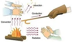
A campfire illustrating the four modes of heat transfer

Heat flows so that the body and the surroundings reach the same temperature, when one system is at a different temperature from another, in order to attain thermal equilibrium. As described by the second law of thermodynamics, this spontaneous heat transfer always occurs from a region of high temperature to the region of lower temperature.

Mechanisms

The fundamental modes of heat transfer are:

• Advection: it is the transport mechanism of a matter, where energy, including thermal energy, is moved by the physical transfer of a hot or cold object from one location to another, and is dependent on motion and momentum of that matter. An example is thermal hydraulics or when wind blows cold air blows in a hot region or vice versa.

• Conduction or diffusion: in this mechanism the heat is transferred, when neighbouring atoms vibrate against one another, or when transfer of electrons takes place from one atom to another. The transfer of heat energy takes place between objects that are in physical thermal contact. Thermal conductivity is the property of a material to conduct heat and evaluated primarily in terms of Fourier's Law for heat conduction.

• Convection: The transfer of thermal energy between an object and its environment, due to fluid motion. Convection is the transfer of heat energy from one place to another through the movement of fluids, a process that is essentially the transfer of heat via mass transfer. Bulk motion of fluid enhances heat transfer in many physical situations, such as between a solid surface and the fluid. Convection is usually the dominant form of heat transfer in liquids and gases.

• Radiation: The transfer of energy by the emission of electromagnetic radiation.

Conjugate Heat Transfer

The Conjugate Heat Transfer (CHT) analysis type allows for the simulation of heat transfer between solid and fluid domains by exchanging thermal energy at the flow interfaces between them. The contemporary conjugate convective heat transfer model was developed after CFD came into wide use. It was used in order to substitute the empirical relation of proportionality of heat flux, to temperature difference, with heat transfer coefficient. This model describes the heat transfer between a body and a fluid flowing over or inside it as a result of the interaction of two objects. The physical processes and solutions of the governing equations are considered separately for each object (i.e. fluid and body) in two subdomains. Matching conditions for these solutions at the interface provides the distributions of temperature and heat flux along the body and flow interface. Typical applications of this analysis type exist as, but are not limited to, the simulation of heat exchangers, cooling of electronic equipment, and general-purpose cooling and heating systems.

Heat Transfer by Solids and Fluids

Heat Transfer in a Solid

Heat transfer in solids, in most cases, is only due to conduction. To describe conduction, Fourier’s law defines the conductive heat flux, q, as proportional to the temperature gradient:

The temperature field in an immobile solid, for a time-dependent problem, is verified by the following form of the heat equation:

Heat Transfer in a Fluid

Due to the fluid motion there are three contributors to the heat equation:

1. The convective contribution, which appears in the heat equation, is due to the transport of fluid, which implies energy transport as well. The dominance of convective or conductive heat transfer depends on the thermal properties of the fluid and the flow regime.
2. The viscous effects of the fluid flow produces fluid heating. This term's contribution is noticeable for fast flow in viscous fluids, otherwise it's neglected.
3. As soon as a fluid density is temperature-dependent, a pressure work term contributes to the heat equation. This accounts for the effects like, producton of heat when air is compressed.

Effective Heat Transfer

Efficiently combining heat transfer in fluids and solids is the key to designing effective coolers, heaters, or heat exchangers.

The fluid usually plays the role of energy carrier on large distances. Forced convection is the most common way to achieve high heat transfer rate. In some applications, the performances are further improved by combining convection with phase change (for example liquid water to vapor phase change).

Even so, solids are also needed, in particular to separate fluids in a heat exchanger so that fluids exchange energy without being mixed.

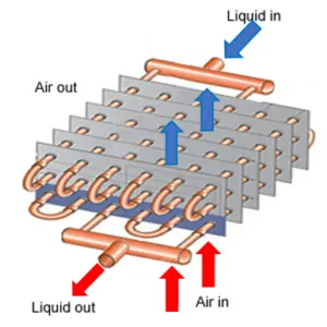
Air to liquid heat exchanger, with metal tube to separate air and liquid(hot air is cooled)

Heat sinks are usually made of metal with high thermal conductivity (e.g. copper or aluminum). They dissipate heat by increasing the exchange area between the solid part and the surrounding fluid.

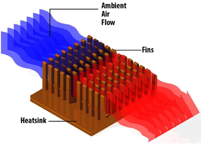
Heat sinks with fins are used to increase the exchange area between the flow and the heat generating components

Use of CHT analysis in industries

Industries that make use of CHT analysis are, but not limited to:

• Automobile industries: for designing the cooling system for engine and gearbox.
• Refrigeration industry: industrial and general-purpose cooling and heating systems.
• Electrical and IT industry: cooling of electronic equipment through liquid or air cooling.

Heat transfer coefficient

The heat transfer coefficient is the proportionality constant between the heat flux and the temperature difference, ΔT.

The overall heat transfer rate for combined modes is usually expressed in terms of an overall conductance or heat transfer coefficient, U. In that case, the heat transfer rate is:

Where:

A : surface area where the heat transfer takes place, m2

T2 : temperature of the surrounding fluid, K

T1 : temperature of the solid surface, K.

The general definition of the heat transfer coefficient is:

where:

q: heat flux, W/m2; i.e., thermal power per unit area, q = d𝑸/dA

h: heat transfer coefficient, W/(m2•K)

ΔT: difference in temperature between the solid surface and surrounding fluid area, K

It is used in calculating the heat transfer, typically by convection or phase transition between a fluid and a solid. The heat transfer coefficient has SI units in watts per square meter kelvin: W/(m^2.(K)).

Selecting turbulence model: K-omega

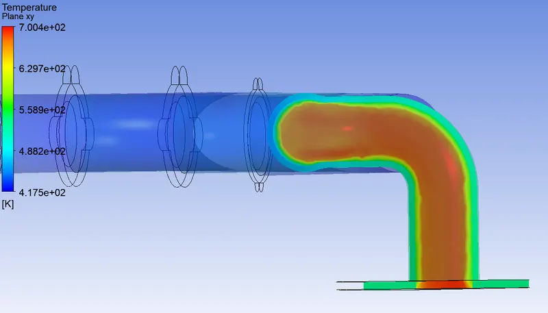
In this simulation we’re conducting a conjugate heat transfer analysis where we’re performing a simulation of heat transfer between solid (exhaust manifold) and fluid (hot exhaust gas) domain by exchanging thermal energy at the interface between them. As exhaust gases flow through the pipe, the pipe gets hot,and in certain areas of the pipe, temperatures are higher than the surrounding, this is due to the velocity of exhaust gases at those areas being higher than the areas where temperatures are lower.

To calculate the flow rate of exhaust air near the inner surface of the pipe accurately, we need to choose a turbulence model that calculates the near wall phenomenon and heat transfer phenomenon correctly. Henceforth we choose the K-omega model for this simulation because the flow demands integrating through the viscous sublayer. The integration through the viscous sublayer is due to the fact that, k-omega model has no-slip boundary conditions, and takes ‘elliptic’ near wall behaviour, which helps the model to interact well with the walls.

The K-Omega viscous model is used widely for simulations that involve heat transfer, calculation of aerodynamic drag, flows with adverse pressure gradients, etc. Integrating through the viscous sublayer would generally impose resolving the mesh to y+<1.

Validating Results:

There are three stages at which heat exchange takes place in the given simulation:

1. The first scenario begins with heat getting transferred from the exhaust gas to the pipe walls through forced convection during fluid flow from the inlets of the manifold to the outlet.
2. The convected heat then travels from the internal surface of the manifold to the external surface by conduction through the solid pipe wall.
3. The conducted heat is then convected to the surrounding, by natural convection as it is assumed that both the model and the air surrounding it are in stationary condition.

In this simulation, we are interested in finding the wall heat transfer coefficient on the internal surface of the pipe and so the heat transfer properties will be evaluated based on the boundary condition assumed for solving the model.

As the Reynolds number calculated for the flow inside the pipe suggests that the flow behaviour is turbulent in nature, The Dittus-Boelter heat transfer coefficient correlation can be used to calculate the Nusselt number which is the ratio of convective heat transfer to conductive heat transfer.

so, Nu=0.023(Re^0.8)(Pr^n)

where,

Pr (prandtl number) = (μ.Cp)/k

μ = fluid viscosity

Cp= specific heat of the fluid at const. pressure= 1075 j.kg/K

k = thermal conductivity of the fluid = 0.0242 W/m.K

n = 0.3

The above equation is also valid for the given boundary condition based on the limitaions defined below

0.6≤Pr=0.0517≤160

Re=58189.896>10,000

(L/D)>10

We know that Nusselt number is Mathematically written as

Nu=h/(k/L)

Where,

L = characteristic length

k = thermal conductivity

h = convective heat transfer coefficient .

Solving for h we’ll get the heat transfer coefficient using thermal conductivity of air as 0.0242 /WmK.

The Dittus-boelter heat transfer coefficient correlation is used here as it was observed to be accurate in the range of ±15% and works best when the pipe surface is very smooth.

Analytical solution:

Assumptions and given data:

Working fluid = air,

ρ = 1.225 kg/m^3 ,

μ = 0.000017894 kg/m.s ,

U = 5 m/s,

L (length of diameter)= 0.170 m,

Y+ value = 0.6, since turbulence model is K-Omega SST.

Calculation:

• Reynolds number :-

Re = (ρVL)/μ = 58189.896

• Skin friction coefficient :-

Cf = (0.026)/(Re)1/7 = 0.005427

• Shear stress near wall :-

𝛕wall = (Cf⋅ρ⋅U^2) /2 = 0.083 N/m^2

• Friction velocity :-

UFric = √((𝛕wall) /ρ) = 0.260

• First layer thickness :-

ΔS = (Y+⋅μ)/(UFric⋅ρ) = 0.000033661 m

• Total thickness of Inflation for 5 layer :-

TotalThickNess = 0.00025 m

Procedure:

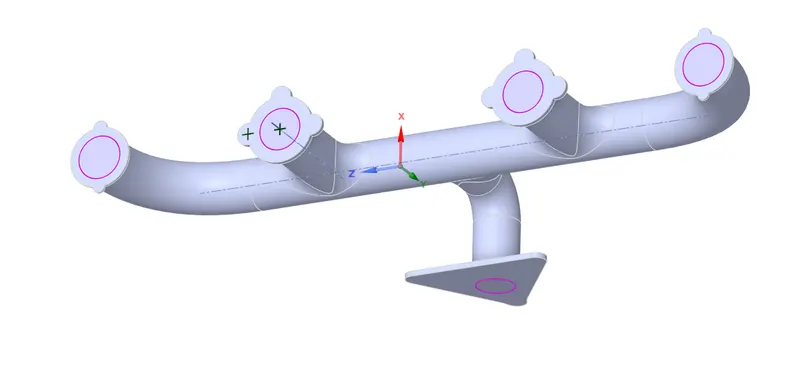
Geometry preparation:

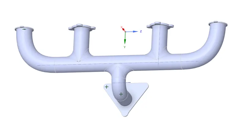
1. Open the part file of the exhaust port provided.
2. Go to prepare and select extract volume and select the inlet and outlet edges.
3. Rename the solid component to “Solid-Volume” and the extracted volume to “Fluid-Volume”, then move these volumes under one component named, “Final-Component” by selecting both and right clicking on the “move to new component” button.
4. Then under workbench select share topography.

Generating Mesh:

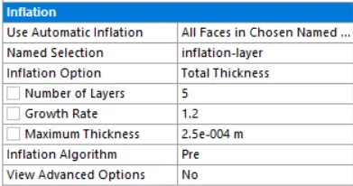
1. Name the sections accordingly, i.e. inlet,outlet, outer-wall-convection, inner-wall and inflation layer. Generate a baseline mesh.
2. Generate inflation layer, on named section “inflation-layer” with total thickness of 0.00025 m and a total of 5 layers.
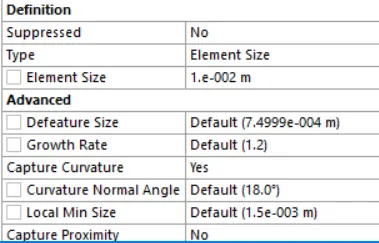
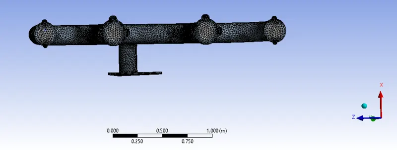
3. The select mesh sizing to refine the solid volume mesh for getting better heat transfer results.

Setup for solving:

1. Select energy equation option, then select K-omega sst model as viscous model, under physics.
2. Then set the boundary conditions of the “inlet”, assign inlet velocity as 5m/s and temperature of the working fluid as 700K. And for boundary “outer-wall-convection”, select convection under thermal conditions and HTC as 20 (w/m^2k).
3. Then under solution to create plots of wall htc and surface htc go to definition>new>surface report>area wtd. Avg., then change the field variable to wall fluxes and under that either select surface htc or wall adj. Htc., then initialize under hybrid method.
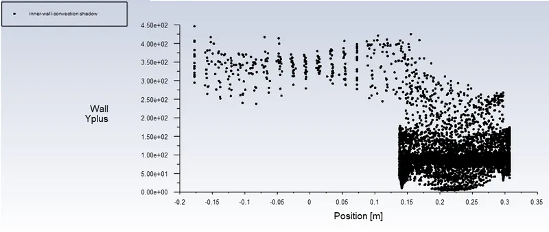
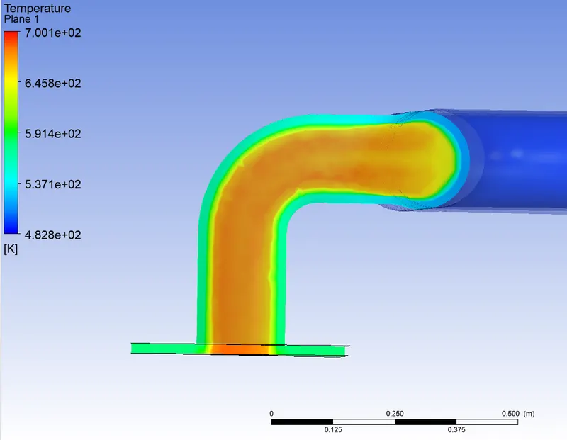
4. Create temperature contour to check the temperature differences over the outer-wall-convection boundary. And create a plot for checking the range of y+ value over the inner-wall.
5. Then run the simulation for 250 iterations.

Post processing:

1. Select outer wall convection named section, change colour to temperature and set the transparency to 0.8.
2. Add an XY plane and colour it with velocity and temperature, then add streamlines from inlet to check the flow of velocity over the interior of the pipe.

Results:

Baseline Mesh Results:

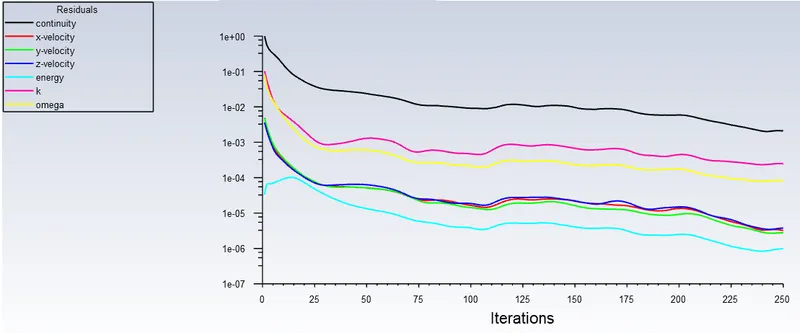
Number of elements=1,37,305

Residuals:

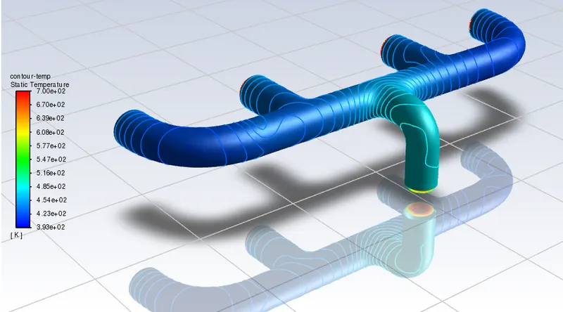
Temperature Contour:

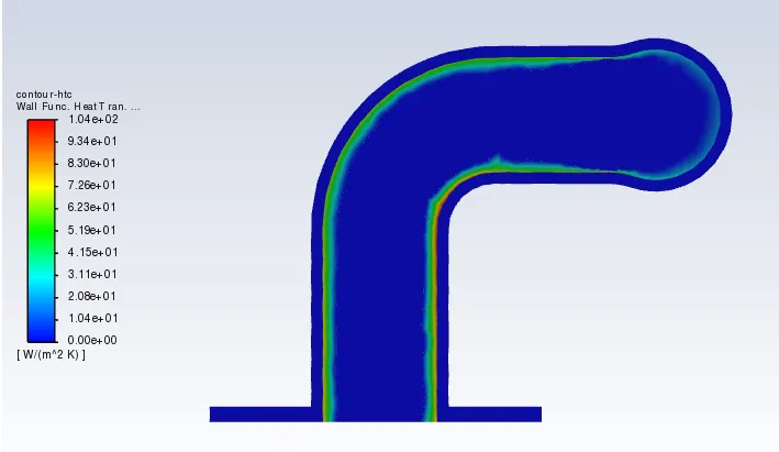
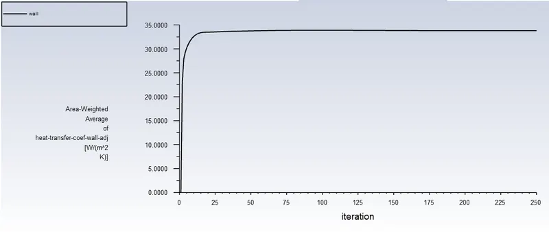
Wall HTC:

Wall HTC value= 33.79 W/m^2.K

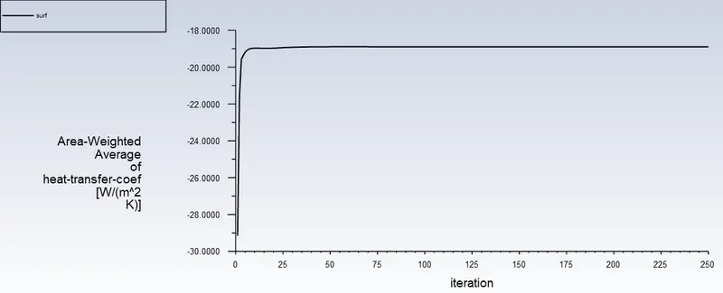
Surface HTC:

Surface HTC value= 18.89 W/m^2.K

Y+ value plot:

Post Results:

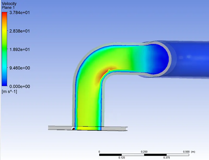
Velocity contour:

Temperature contour:

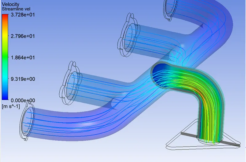
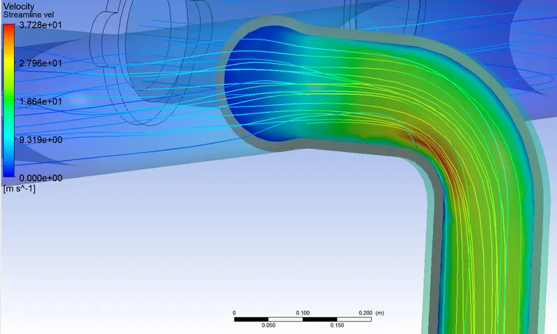
Streamline:

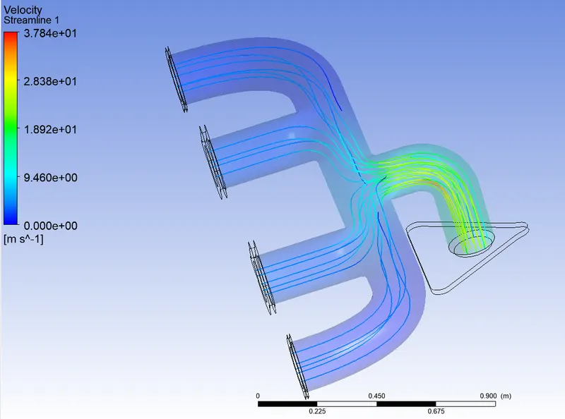
Refined Mesh Results:

Number of elements=4,09,145

Residuals:

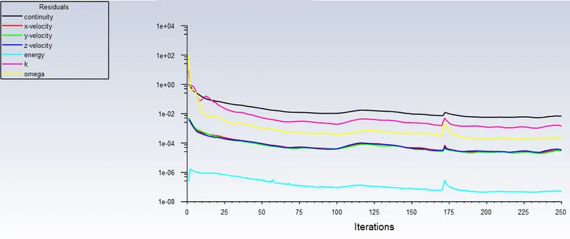
Temperature Contour:

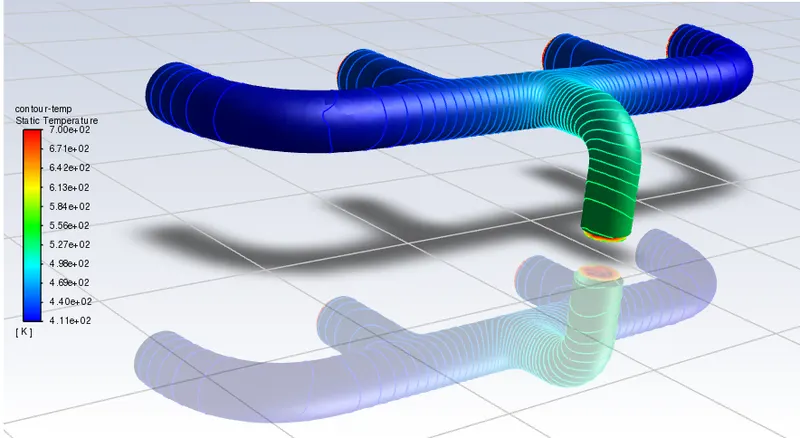
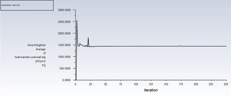
Wall HTC:

Wall HTC value= 1445 W/m^2.K

Surface HTC:

Surface HTC value=18.5 W/m^2.K

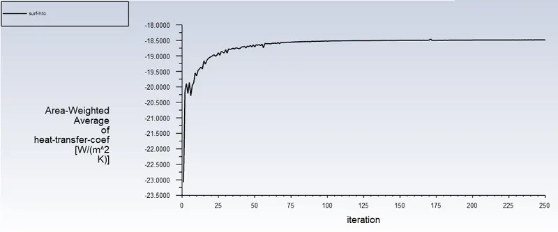
Y+ value plot:

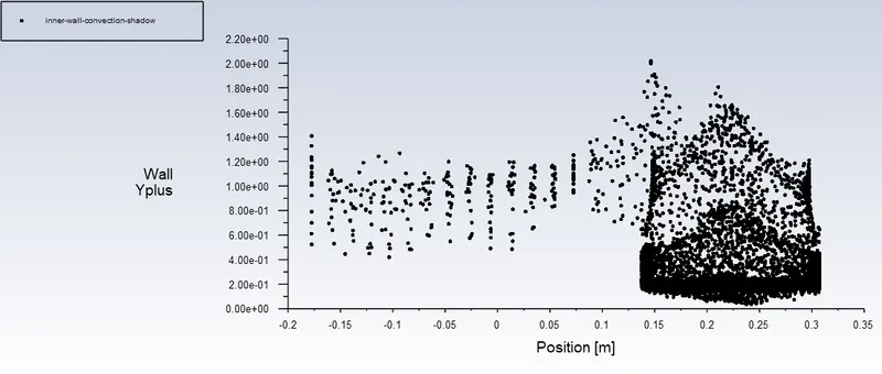
Post Results:

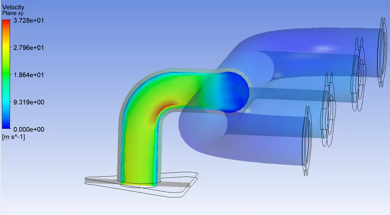
Velocity contour:

Max vel.=37.27 m/s

Temperature contour:

Streamline:

Observation:

1. The effect of element size can be clearly observed in two cases.
2. Results are more accurate and near to exact values with finer mesh.
3. In case of refined meshing we introduced "inflation layers" , because of that there is a drastic change in the wall HTC .
4. Remaining Values are not that much effected .
5. The velocity streamline starting from the inlets is shown , where the velocity is low in the inlet sections and higher at the outlet section , this is because of mass conservation.

Inference:

Hence, CHT analysis on exhaust port was conducted.