Week 4 - CHT Analysis on Exhaust port
Conjugate Heat transfer (CHT) analysis on exhaust port
Aim : To perform a CFD simulation on an exhaust port and determine the Surface heat transfer coefficient on the internal solid surface of the exhaust port.
Objective(s) : 1. Provide a reson for the higher magnitude of surface heat transfer coefficient near to the wall.
2. Provide the factors on which the Heat transfer coefficient depends
3. Validating the result with the available literature.
Theory:
Conjugate heat transfer :
In general, when a heat transfer takes place, it is through the methods of conduction, convection and radiation simultaneously. However, the conduction mode of heat transfer dominates in solids. Likewise, in gases the convetion/ radiative heat transfer dominates. In liquids, either the convective or the conductive method dominates.
Some common examples where conjugate heat transfer analysis if performed are :
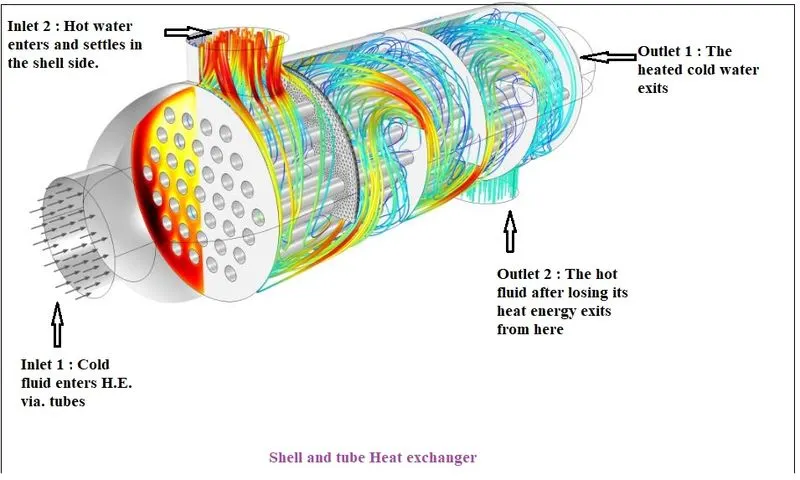
1. Heat exchanger analysis : Consider a shell and tube heat exchanger where heat from the fluid at high temperature is transferred to the fluid at low temperature. In the process, heat gets transferred from hot fluid to the walls of the tubes and to the cold fluid. The processes happeining here are convective heat transfer from hot liquid to the walls, conductive heat transfer from face of the wall in contact with the hot fluid and convective heat transfer from other face of the wall to the cold fluid.
2. Heat sink : A heat sink is a passive heat exchanger that transfers the heat generated by an electronic or a mechanical device to a fluid medium, often air or a liquid coolant, where it is dissipated away from the device, thereby allowing regulation of the device's temperature. In computers, heat sinks are used to cool CPUs, GPUs and some chipsets and RAM modules. Heat sinks are used with high-power semiconductor devices such as power transistors and optoelectronics such as lasers and light emitting diodes (LEDs), where the heat dissipation ability of the component itself is insufficient to moderate its temperature. [1]
Priciple of working :
Based on the law of thermal conductivity `Q = -k*A*(dt)/(dx)`and Newton's law of cooling `Q = h*A*Delta(t)`, an increase in the area of heat dissipation increases the rate of heat transfer. A heat sink does exactly that i.e., it increases the area of heat transfer.
In general the heat sinks are made of high thermal conductivity materials like copper and aluminium.
For example consider a heat sink intsalled on the processor of a circuit board.
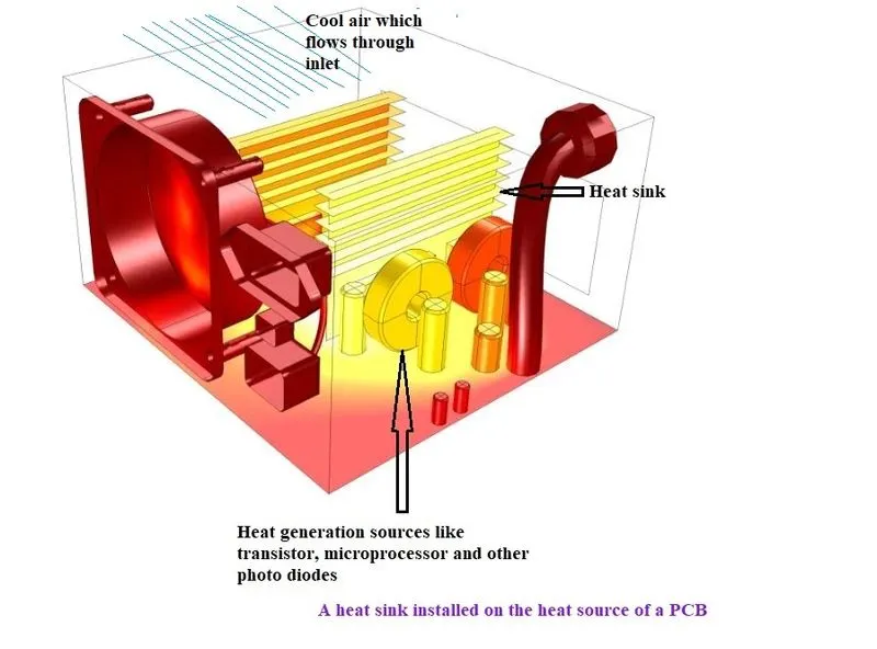
The cool air which blows over the heat sink extracts the heat from it as it is at higher temperature. Here, the mode of heat transfer is conduction. Also, the heat generated by the processor is transferred to the heat sink by the process of heat conduction. This is the perfect example of conjugate heat transfer.
Need for the Conjugate heat transfer analysis :
In order to determine the conductive heat transfer coefficient (K) as well as the convective heat transfer coefficient (h), a conjugate heta transfer simulation is necessary. This helps in the determination of the dominant mode of heat transfer in that particular heat transfer problem.
-------------------------------------- - - --- --- -------------------------- ---- --- ----- -- -- ---------- ----------------------- ----- -------------------- ---- -
Setting up the CFD simulation :
1. Geometry preperation :
The pre modelled geometry of the exhaust port is imported into the SpaceClaim module of the ANSYS workbench. Here the fluid domain and the solid domain are separated by using the voulme extraction tool of SpaceClaim. The share topology option is to be enabled which is important for the ANSYS Mesher to identify the components and generate a conformal mesh.
A confromal mesh is one where the elements of two meshes intersect only at point or an edge. This means there should be no intersection area.
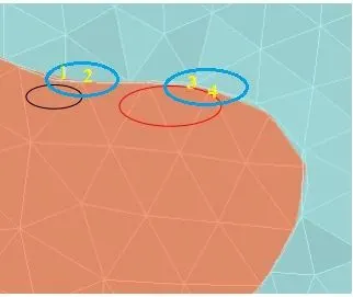
Fig : Non conformal mesh
In the above figure point 1 lies on the green mesh whereas point 2 lies on the orange mesh surface. For the conformal mesh,the point 2 and point 1 should coincide.
The following is a screenshot of the conformal mesh :
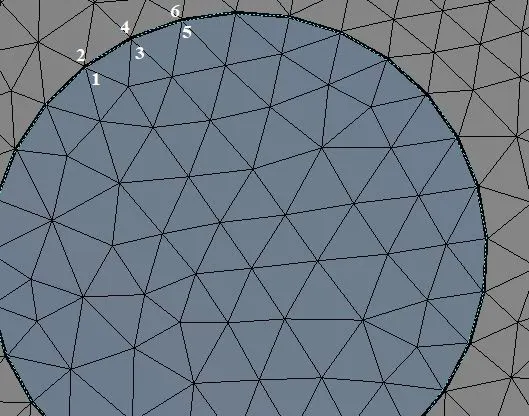
Fig : Conformal mesh
Here, the points 1 &2, 3 & 4, 5 & 6 coincide exactly.
Mesh details :
| S.No | Number of elements | Number of nodes |
| Basic mesh | ||
| Refined mesh 1 |
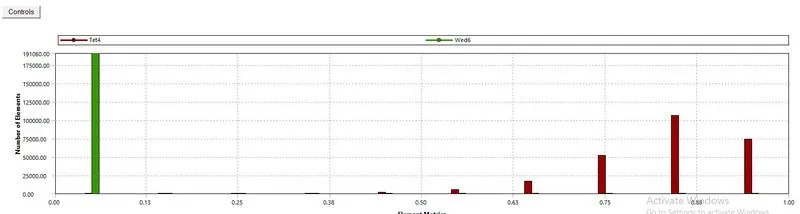
Mesh Metrics :
Concept of Y Plus :
The Y plus is a dimensionless quantity. It is a distance measured normal to the wall in terms of viscous lengths.
The exact need for the Y plus is to distinguish different regions near the wall like Viscous sublayer, buffer layer, ovelap layer and turbulent layer.
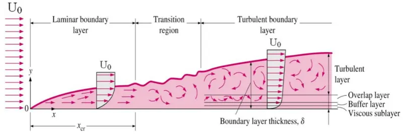
In order to clearly resolve the boundary effects the cells near the mesh near the wall should be fine. However, this has the effect of increasing the cell count and computational cost.
So we use the option of adding the inflation layers. But the questions which arise are : What would be the size of the first cell near the wall ? What would be the total thickness of the inflation layers ?
In order to answer this knowledge on determination of Y-plus value is must which begins with the calculation of first cell height.
The definition of `y+`is such that `y+ = (rho*U_tau * Deltay_1)/(mu)`
Rearranging the above equation for `Delta y_1`gives `Delta y_1 = (y+*mu)/(rho*U_tau)`
Here, `Delta y_1`is the first cell thickness
`U_tau`is the frictional velocity
Steps to calculate the first cell height :
1. Determine the value of the Reynolds number.
`Re = (rho*v*L)/(mu)`. Here V is the flow velocity, `rho`is the fluid density, `L` is the characteristic length and `mu`is the absolute viscosity.
2.
As per the definition of yplus
`y+ = (rho*U_t*Dely_1)/mu`
Rearranging for `Delta y_1` we get
`Delta y_1= (y+* mu)/(rho*U_t)` -----(a)
where, `U_t` is the frictional velocity which can be calculated by the formula:
`U_t = sqrt((tau_w)/(rho))`
`tau_w` which is the wall shear stress can be calculated from the skin friction coefficient `C_f` as `tau_w = 1/2* C_f* rho*U^2`
The empirical value of skin friction coefficient is as follows:
`C_f = 0.079*Re^(-0.25)`, for internal flows and`C_f= 0.058*Re^(-0.2)`, for external flows.
Upon inputting the calculated value of `U_tau` in the formula for `Deltay_1` we obtain the first cell height.
Calculation of Y-plus value for the geometry :
The chosen y plus range is from 0.3 to 1.5 as the turbulence model used for solving the case is `k-omega. It is an established fact that `k - omega`works well with the low range of Y-plus values starting from 0 to 5.
Case setup in FLUENT :
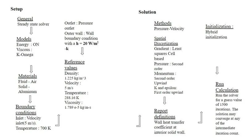
Results :
The analysis has been done for the y+ values of 0.5,1,1.3 and 1.5.
Case.1 : Using the `k-omega`turbulence model with y+ of 0.5
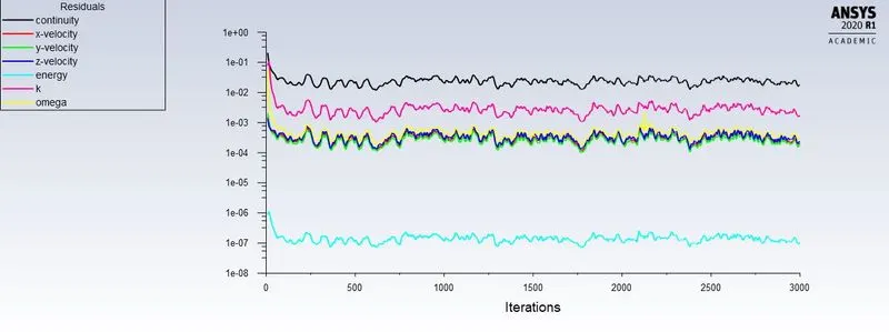
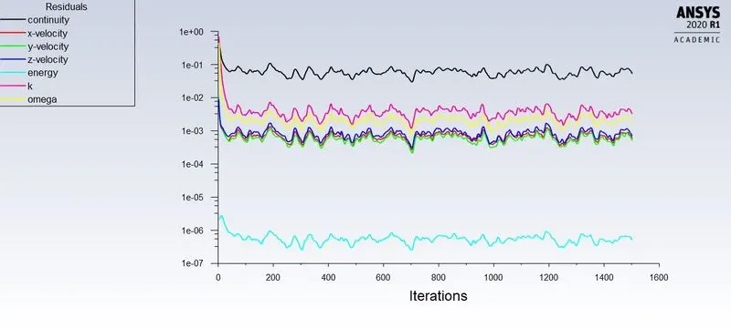
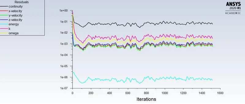
Residuals plot :
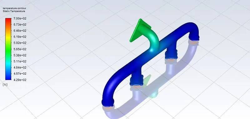
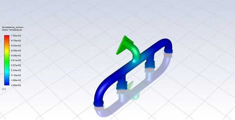
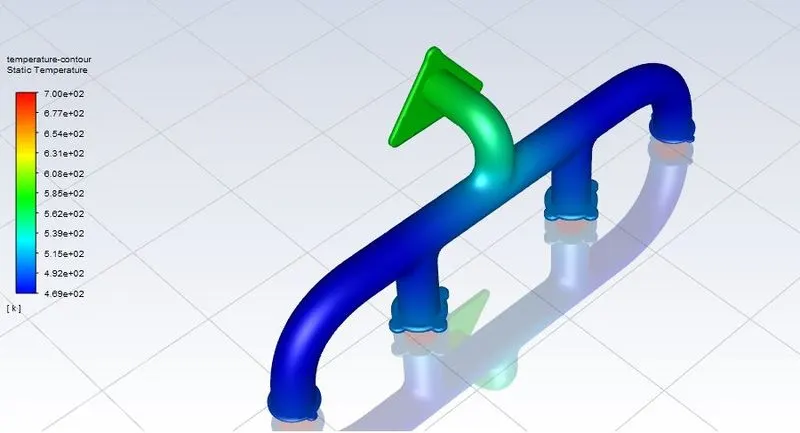
Temperature contour :
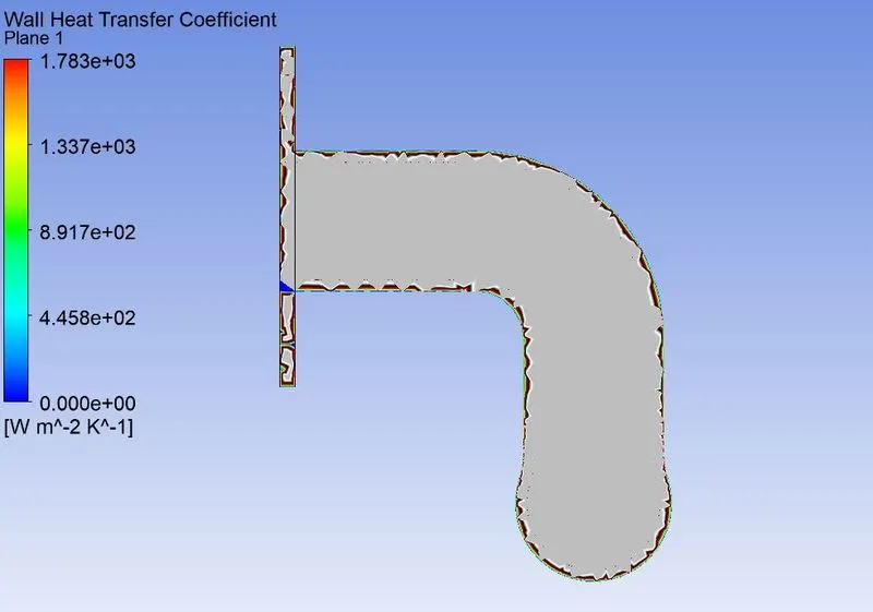
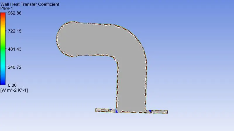
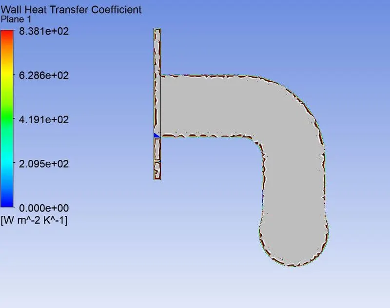
Wall heat transfer coefficient :
It can be observed that the wall heat transfer coefficient is highest on the surface of the internal solid wall.
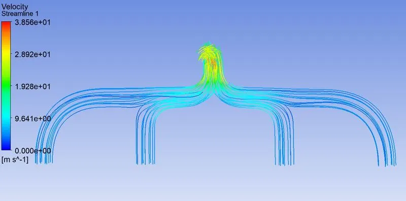
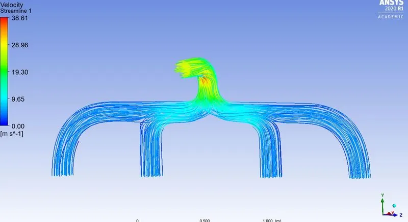
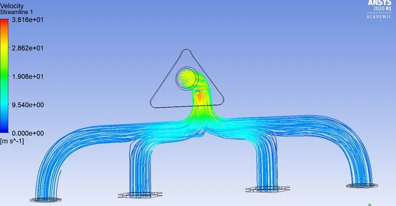
Streamlines of velocity plot :
Case 2 : `k-omega`turbulence model with y+ value of 1
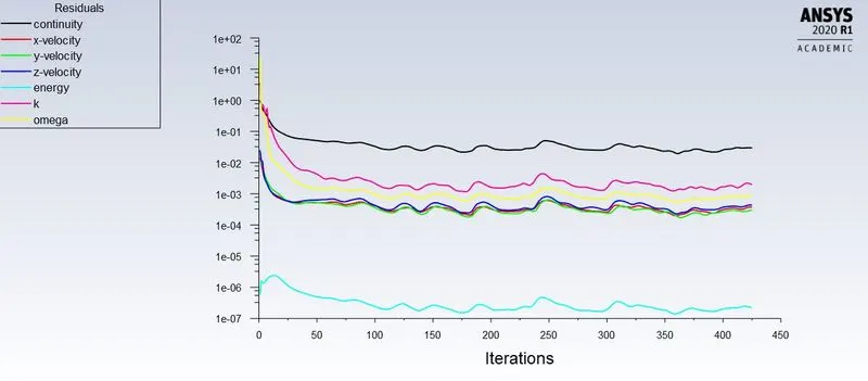
Residuals plot:
Temperature contour plot :
Wall heat transfer coefficient :
Streamlines of velocity plot :
Case. 3: `k-omega`turbulence model with y+plus value of 1.3
Residual plot :
Temperature contour plot :
Wall heat transfer coefficient plot :
Streamlines of velocity plot :
Case. 4 : `k-omega`turbulence model with y+ value of 1.5
Residual plot :
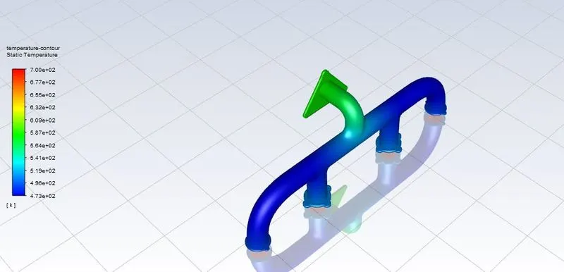
Temperature contour plot:
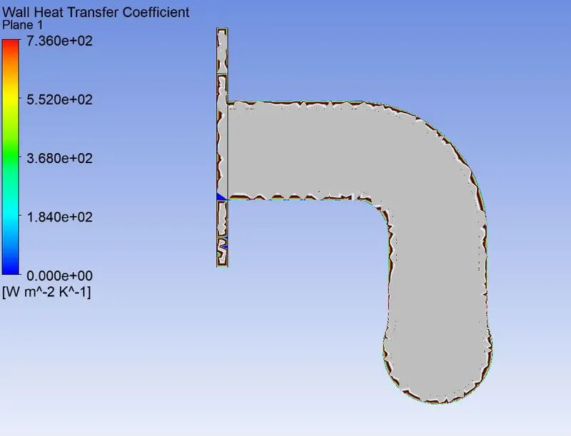
Wall heat transfer coefficient plot :
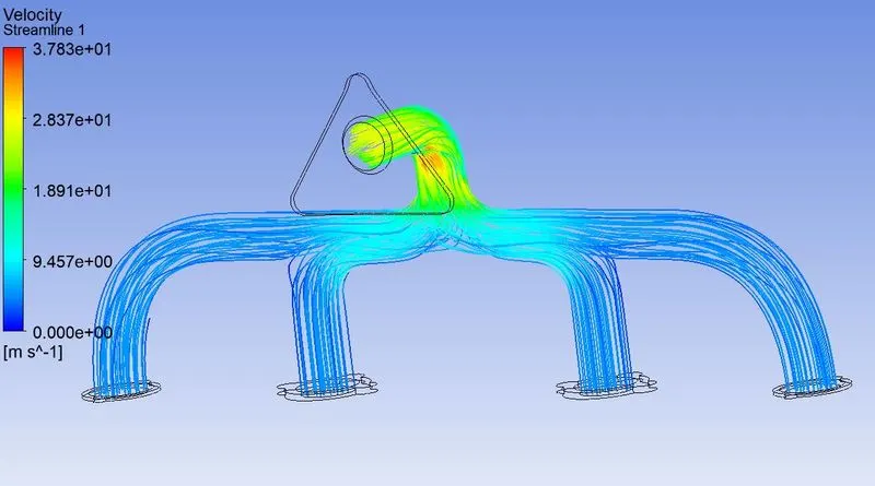
Streamlines of velocity plot :
Tabular form of the obtained results :
| Number of the cells | Y-plus | Wall heat transfer coefficient (`W/(m^2-k)`) | Outlet temperature (`T_(out)`) |
| 446,457 | 0.5 | 1690. 923 | 628.33 |
| 446,128 | 1 | 847.489 | 580.2 |
| 444122 | 1.3 | 654.38 | 679.25 |
| 443,441 | 1.5 | 679.34 | 679.25 |
Analysis of the results :
It can be observed that the wall Heat transfer coefficient value for the case of y+ value of 1 is 847.489 `W/(m^2-k)`. This lies in the expected range of 800 - 1200 `W/(m^2-k)`.
Verification of the results from the simulation:
1. The wall heat transfer coefficient is maximum at the wall and it is non existent at the other areas of the geometry. It is evident from the wall heat transfer coefficient contour plot that wall HTC is maximum at the wall.
2. The velocity is maximum at the mid streamline of the fluid.
3. Flagging the boundaries correctly as well as defining the solid and fluid regions correctly is one more important factor for accurate CHT simulation
Conclusion:
A CHT simulation on the exhaust port of an automobile is performed and the wall HTC is determined.