Week 4 - CHT Analysis on Exhaust port
AIM: To simulate Conjugate Heat Transfer Analysis of an Exhaust Manifold in ANSYS FLUENT.
Introduction:
Exhaust Manifold is used across industries where combustion is the primry mode of power production. The main purpose of this device is to capture and deliver emissions as required. In Automotive industry however, it holds special importance.It is not only a medium that provides a path for exhaust gases but is also aids the catalytic converter which is responsible to ameliorate the harmful emissions present in the exhaust gases.
Catalytic Convertors put the exhaust gases under REDOX reaction, where the more harmful molecules of NO, CO etc are converted into less deleterious ones like NO2, CO2 etc. For successful conversion, the exhaust gases must be at an optimum temperature. If temperature of exhaust gases is too high as it is when they are expelled from the cylinder, these hot gases can damage the catalytic convertor. On the other hand, if temperature of exhaust gases is too low (COLD START) the catalytic convertors do not get activated and harmful exhaust is expelled in the surrounding. The time period at which the catalysts become active is called the Light-Off-Time [1].
This way, exhaust manifold forms a critical component in exhaust assembly of an automobile. The design of its surface must be such that the Total Heat Transfer from the exhaust Manifold must keepsthe exhaust gases under optimum temperature throughout operation of automobile.
| Function | Target Exhaust Temperature deg_C |
| Hydro Carbon Desorption | >200 |
| Desulfation | >400-650 |
| Ammonium Sulphate Removal | >280 |
| Hard Urea Deposit Removal | >400-500 |
| Soot Oxidation in DPF |
250-350 with NO2 > 550 with O2 |
Table 1: Examples of Different Catalysts Regeneration Function and Required Exhaust Temperature [2]
Theorey:
Because of the nature of Heat Transfer process Conjugate Heat Transfer Analysis is required. The overall Heat transfer is obtained by convection between the flowing hot exhaust gases and surrounding wall as governed by Newton's Law of Cooling, then in between the solid through conduction which is Governed by Fourier's Law of Heat Conduction and then again by convection between the outer surface of the exhaust manifold and ambient air.
Fourier's Law of Heat Conduction:
According to this law the rate of Heat flux is directly proportional to gradient of temperature in Space
d/dt (q/A) ∝ ∇.T
= -k ∇.T
where, k is constant of proportionality called thermal conductivity of the material which is a property of solid. [w/mK]
q is the amount of heat transfered [j]
Newtons Law of Cooling:
The rate of heat flux between a flowing fluid and stationary solid is given by,
d/dt (q/A) ∝ (T(fluid) - T(solid))
= -h*A*(T(fluid) - T(solid))
where, h is constant of proportionality called convection heat transfet coefficient. [w/mK]
h = f(thermophysical properties of the fluid, velocity of the fluid)
=> if anywhere in the computational domain velocity increases, the heat transfer coefficient must also increase
Calculation of Reynolds number
For internal flows we have an estimate of Reynolds number with subsequent flow behaviour, the flow can deviate from this estimate with regards to geometry and flow conditions, but for the most cases including ours, this estimate is acceptable [3]
| Reynolds Number Range | Flow Behaviour |
| 0<Re<1 | Highly viscous Creeping Flow |
| 1<Re<100 | Laminar flow |
| 100<Re<1000 | Laminar Boundary layer flow |
| 1000<Re<10000 | Transition to Turbulence |
| 10000<Re<10000000 | Turbulent flow |
Table 2: Reynolds number and flow behaviour
Calculation
Re,d=ρ*V*d/u
ρ = 1.225 kg/m^3, density of air at free stream temperature of 300 K
u = 1.789*10^-5 Pa*s, absolute viscosity of air
V = 5 m/s, velocity of air
d = 0.166 m, diameter of inlets and outlet
Re,d = 5.68*10^4
Since Re>10000 => FLOW IS TURBULENT
Due to the complexity of the geometry the ∇.T term can not be solved by analytical techniques and thus Numerical Methods are needed.
We are not going to model the convective heat transfer between outer surface of the exhaust manifold and the ambient air due the excessive time and computational cost associated with it.
Solving and Modelling Approach:
This geometry is a simplified model of an Exhaust Manifold of an automobile. As discussed in the introduction, the rate of heat transfer from it must be optimized for proper functioning of the Catalytic Convertor. After running the simulation we can estimate the distribution of temperature from its surface and thus how it is expelling the of exhaust gases. The whole idea is to get an insight into the flow of exhaust gases inside the exhaust manifold. This work can lead us to understand the relation between geometry and heat transfer crucial for practical purposes.
Modelling approach is simple and can be classified as the CFD Analysis of internal flows where Conduction and Convection conjugated to slove for the Temperature Flow field that results into evaluation of parameters like convection heat transfer coefficient and rate of heat transfer.
Selection of Turbulence Model with appropriate near wall treatment is critical for results to be in acceptable range.
Turbulence Model
For Turbulence Models we have two options
1. K-Omgea (2 eq) SST which is the default turbulence model in FLUENT and is ideal for simulating flow seperation and adverse pressure gradient based flow.
2. K-ε (2 eq) standard/Relizable: It is used when turbulence is not the main driving factor of flow behaviour and makes it suitable for low to moderate Reynolds number flows
Near Wall Treatment Method
There are two major methods:
1. Scalable wall functions: Used if Reynolds number is high and there is no flow seperation and first layer thickness is such that y+ falls in the log mean layer.
2. Enhanced Wall Treatment: It is a y+ insensitive method and automatically adjusts in accordance to value of y+, if y+ == 1, then it resolves the viscous sublayer, if y+ >>1 then it uses wall functions.
Different Approaches for Near Treatment method
1. Viscous Sub-Layer Resolution: Entire bpundary layer including viscous sub-layers resolved within the mesh. This approach is most appropriate for flows experiencing adverse pressure gradients and flow saperation. This will require to have a y+ = 1, so that the grid point will lie within the viscous sublayer. This requirement imposes higher number of elements and thus slows down the computational process.
2. Logarithmic based Wall-functions approach: In this method we place the first grid point in the outer turbulent region. This approach can incorporate much higher values of y+ ranging from 30>y+>300, if Re is higher, even greater value of y+ is acceptable. But, it is only suitable for flows having favourable pressure gradients.
Because of the value of Reynolds number == 50000 the flow is not highly turbulent and thus viscous stresses might still play a significant role in in the values of wall functions like surface heat transfer coefficient and wall shear stresses.
Y+ and First Layer Thickness:
We will target a Y+ value = 10 and determine the value of first layer thickness needed.
Calculation
Re,d = 5.68 * 10^4
u+ = u/uτ
uτ = (τw/ρ)^0.5
y+ = y*ρ*uτ /μ
where:
uτ = friction velocity
τw = wall shear stress
u+ = dimensionless velocity
y+ = dimensionless distance from wall
Cf = friction factor
We can use flat plae formulae to calculate all these values, since the law of the wall is universal and u+ = f(ln|y+|) is same for all internal and external flows
from flat plate analytical data
τw = 0.5*Cf*ρ*U^2
Cf = 0.058*Re^-0.2 = 0.00588(5.68 *10^4)^-0.2 = 6.495*10^-3
=> τw = 0.5*Cf*ρ*U^2 = 0.0995 Pa
=> uτ = (τw/ρ)^0.5 = (0.0995/1.225)^0.5 = 0.28 m/s
=> u+ = u/uτ = 5/0.28 = 17.55
=> y+ = y*ρ*uτ /μ
=> y = μ*y+/ρ*uτ = 5.124*10^-4 since its the height from wal to centroid of first cell we need to double it to get first layer thickness
=> First layer thickness = 2*y+ = 1.025 mm => 1 mm approx
Convergence Parameters
There are two criterion we can lay emphasis on which can can indicate a convergened solution.
1. Mathematical Convergence: If our residual levels are falling below 10^-3 we can say that the solution is converged mathematically. This generally indicates the accuracy with pre-processing.
To claim mathematical Convergence we will test the following variables in our solver:
1. Area-Weighted Average of Output Temperature = The output temperature from exhaust manifold, if graph shows a straight line then this varable is accurately predicted
2. Mass Balance = Continuity Equation Balance, the result must be negligible => (mass flow rate)output - (mass flow rate)input
3. Area-Weighted Average of Surface Heat Transfer Coefficient = The surface heat transfer coefficient will vary across the domain but a weighted area average will give an average value which if converged will be a closely approximated result.
2. Physical Convergence: If the results obtained are in line with the flow physics then we can cliam physical convergence. For this we have to check contours of temperature, Velocity and surface heat transfer coefficient and the behaviour must not deviate from what is expected, such as if the contour shows higher velocity at a particular location then as per Energy Equation the Pressure must be lower and surface heat transfer coefficient must be higher.
Selection of Turbulence Model with Near Wall Treatment
Due to the nature of the problem we use:
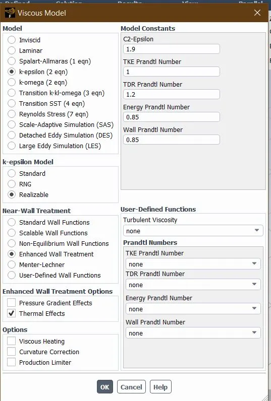
K-ε (2 eq) Relizable with Enhanced wall Treatment and emphasis on heat tranfer
Since we are investigating internal flows with emphasis on heat transfer coefficient we need to select the appropriate Y+ value which will lead to perfect first layer thickness and will eventually result in acceptable results.
We will first run a Baseline Mesh with standard solver settings and then as per the changes required we will refine the mesh and if needed modify the solver settings as well
We will use the following steps to tackle this problem:
Step 1: Simulation on Base line Mesh
Step 2: Improvising the mesh taking reference from Base line results
Step 3: Improvising the mesh further to deduce Mesh Independence test
Step 4: Post-Processing of Results
Step 5: Validation of Results
Gerenal Steps Involved for all Cases
1. Geometry Cleanup in SpaceClaim
This involves setting up the fluid and solid volume and connecting them as common interface with Share command in Workbench
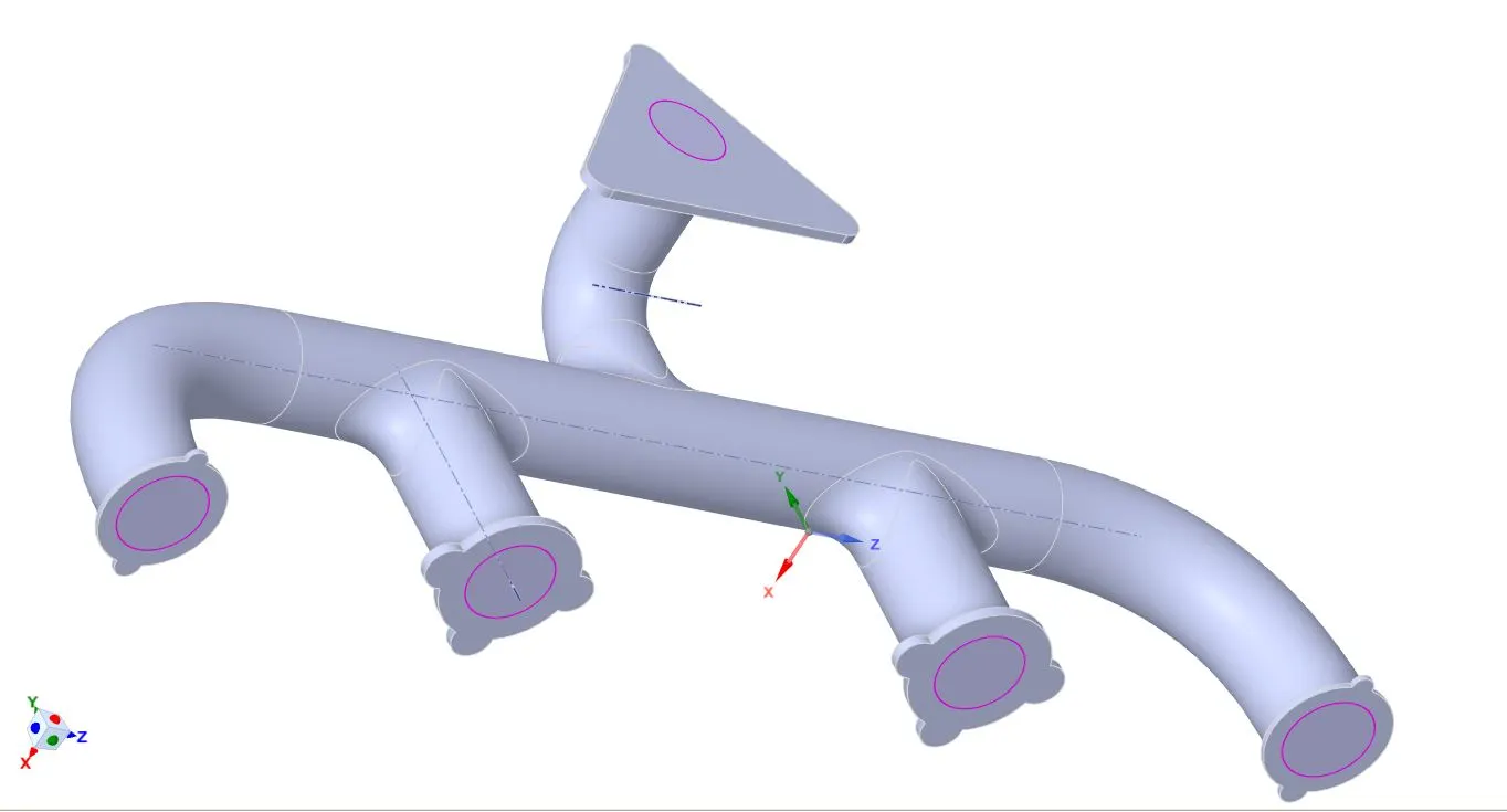
Figure 1: Physical Domain
2. Unstructured Meshing in MESHING tool of ANSYS
Now we mesh the geometry with unstructured tetrahedral elements.
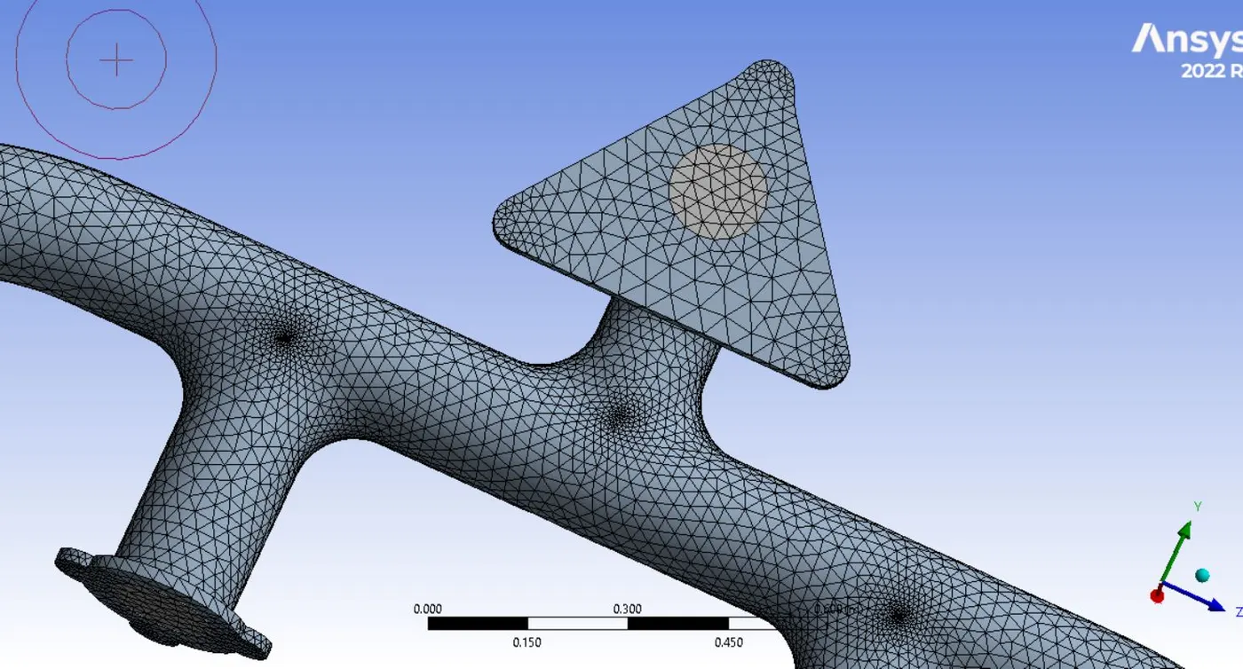
Figure 2: Computational Domain
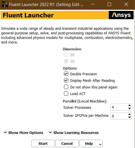
3. Setting up Fluent
4. Setting up solver Settings
5. Running the Solver
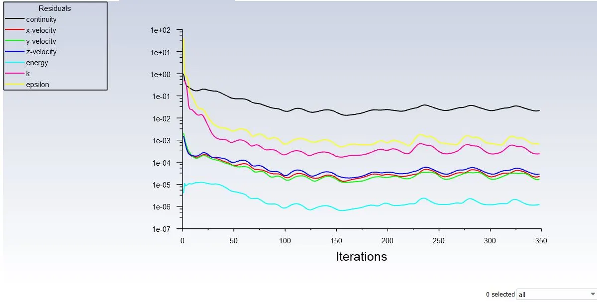
Figure 3: Residuals for Baseline Mesh
As we can see, the residuals are not depicting a proper mesh setup, thus we will refine the mesh.
Step 2: Refining the mesh
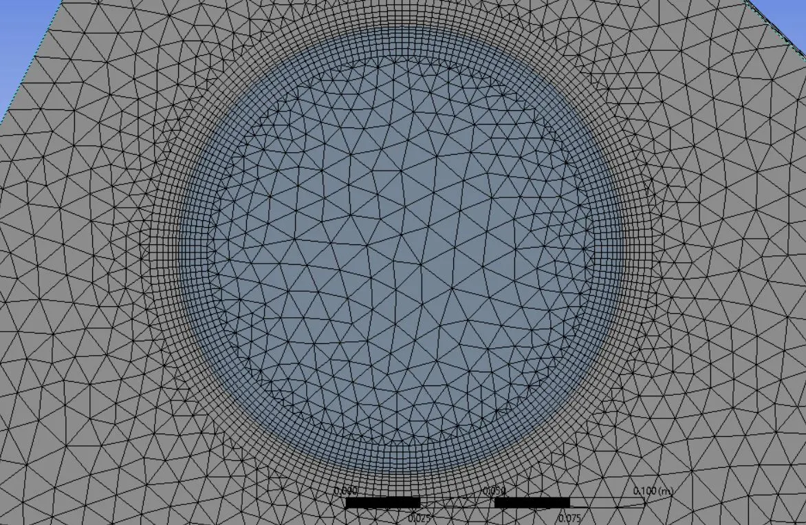
Figure 4: Refined Mesh with Inflation Layers
We have now incorporated sufficient inflation layers to capture the steep variation of the velocity field near wall. But we must ensure that transition from inflation layers to other elements is smooth otherwise the mesh quality will decrease.
Checking the Quality of Mesh
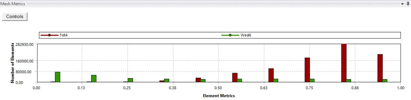
Figure 4: Element Quality
We can see our mesh quality is sufficient to start the solver procedure again
Running the Solution
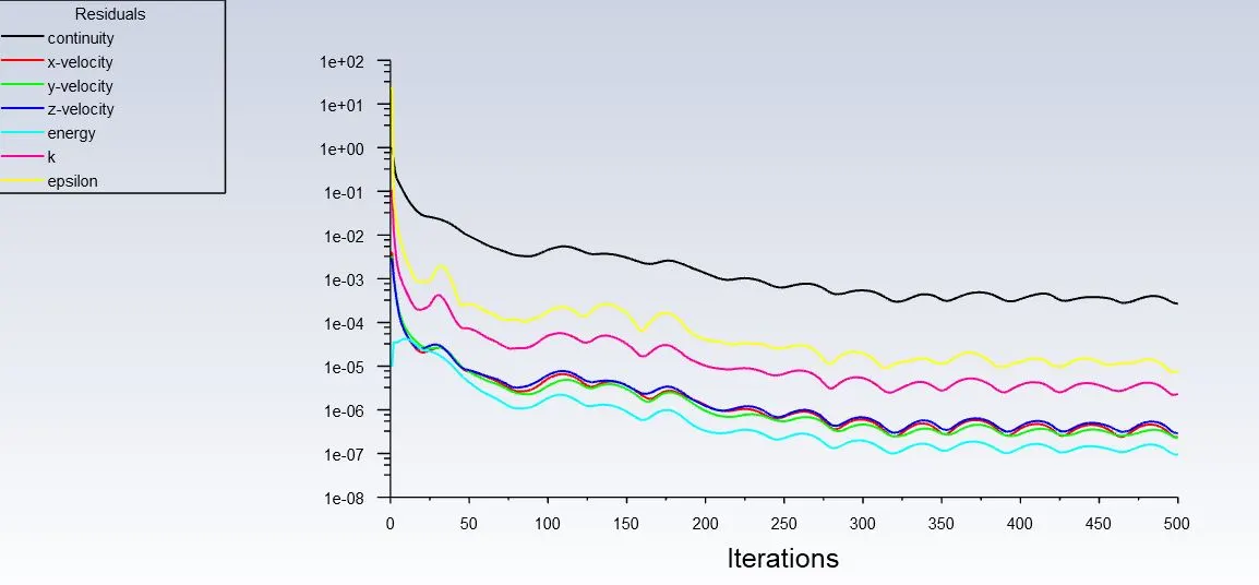
Figure 5: Residuals for Refined mesh
The residuals are below e-3 had thus indicate a accurate setup.
Area Weighted Average of Temperature Outlet
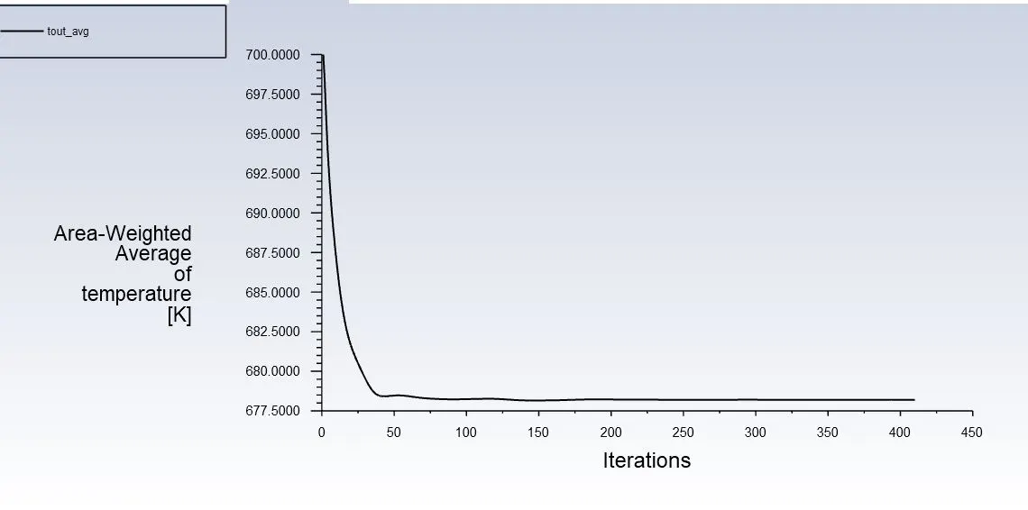
Figure 6: Area Weighted average of Temperature = 678.197 K
Mass Balance
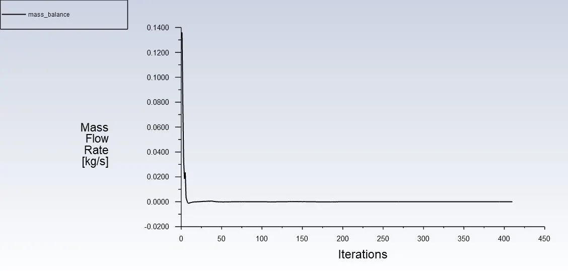
Figure 7: ∆ṁ = 2.01 * 10^-6
Now we will further improve the mesh and check these parameters, if parameters are close to each other then we can proclaim that our setup is mesh independent
Step 3: Refining the Mesh Further
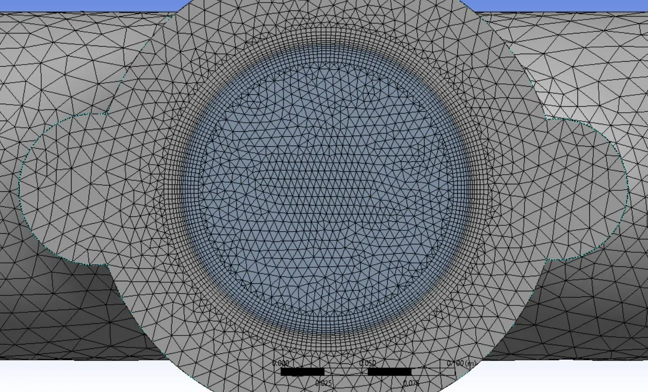
Figure 8: Highly Refined Mesh
As we can observe, our mesh is highly refined with very gradual variations in element sizes across boundries, this will improve the mesh quality further.
Checking the Mesh Quality
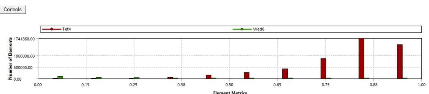
Figure 9: Element Quality of highly refined Mesh
Running the Solver
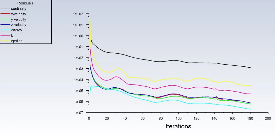
Figure 10: Residuals for Highly Refined Mesh
As we can see, the residuals are continously dropping, we should run the simulation further until a straight line is observed, but due to the time required for this highly refined mesh computation, we limit it upto here.
Average Weighted average of Temperature at outlet for highly refined mesh
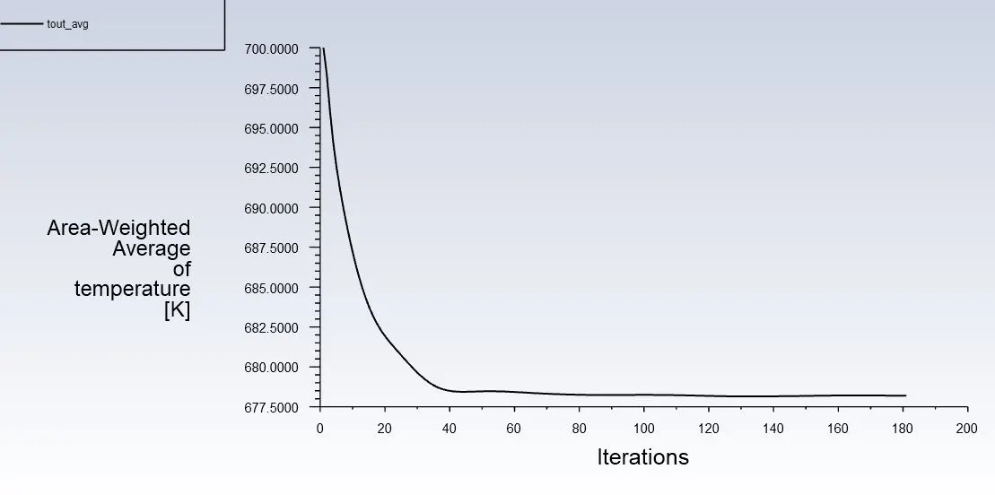
Figure 11: Area Weighted average of Temperature = 678.199 K
Mass Balance for highly refined mesh
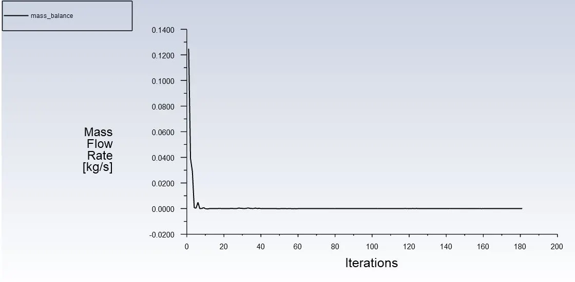
∆ṁ = 3.956 * 10^-6
Now we can summarise our results:
| MESH | NO. OF ELEMENTS | AVERAGE MESH QUALITY | AREA WEIGHTED AVERAGE OF TEMPERATURE OUTLET |
| Baseline | 138404 | 81.86% | 681 K |
| Refined | 1.14 Million | 68.5% | 678.197 K |
| Highly Refined | 5.21 Million | 78.84% | 678.199 K |
Table 2: Summary of Post Processing
Step 4: Mesh Independence Test
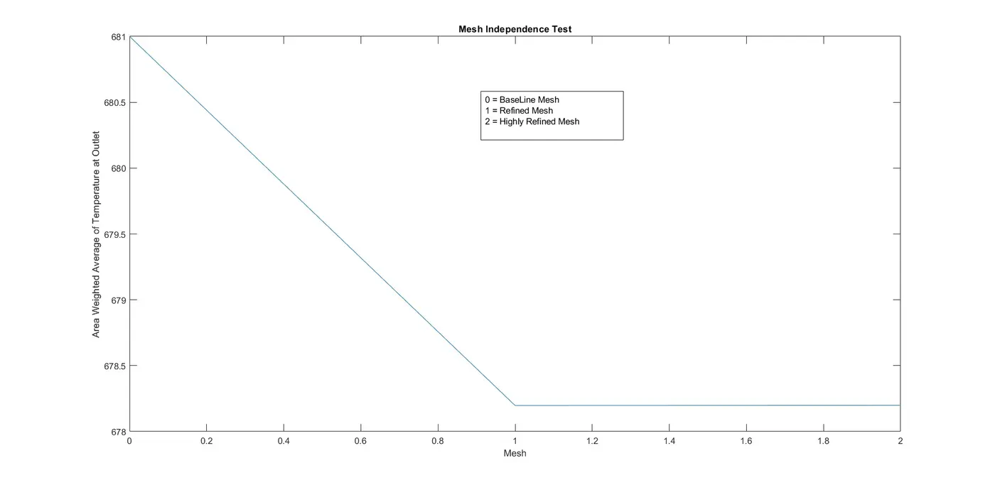
Figure 12: Mesh Independence Test
Now we can see our post processing is leading to a mesh which is inependent of refinement and thus we can work on the results now for post processing
Step 5. Post Processing the results
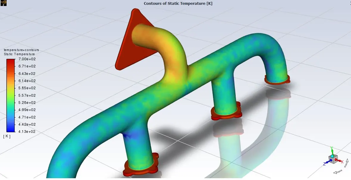
Figure 13: Temperature Contours of Exhaust Manifold
Variation of Temperature, Velocity and Surface Heat Transfer Coefficient
As we can see, the temperature at the outlet portion looks higher than the other regions. We will try to explain this phenomena in accordance to continuity equation and other known physical principles.
1. At inlet Cross-Section
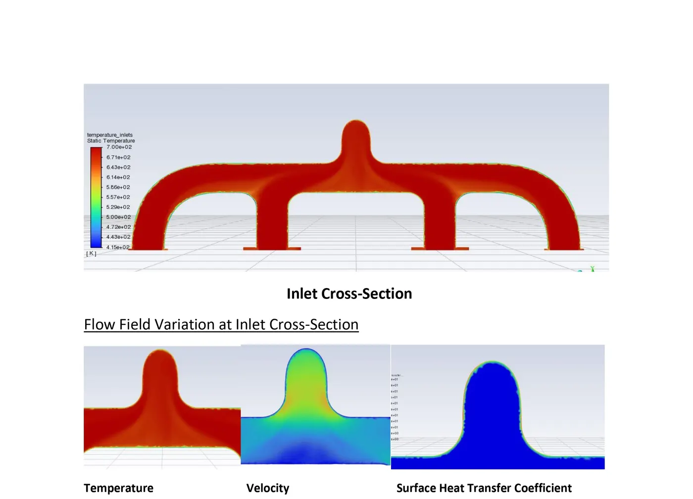
Figure 14: Flow variables varying at inlet Cross-Section
As we have only one outlet, thus to conserve the continuity equation, the speed of the flow increses near the outlet. This increase in velocity will result in increase of surface heat transfer coefficient and thus temperature will also increase.
2. Change in flow geometry effect on flow field variables
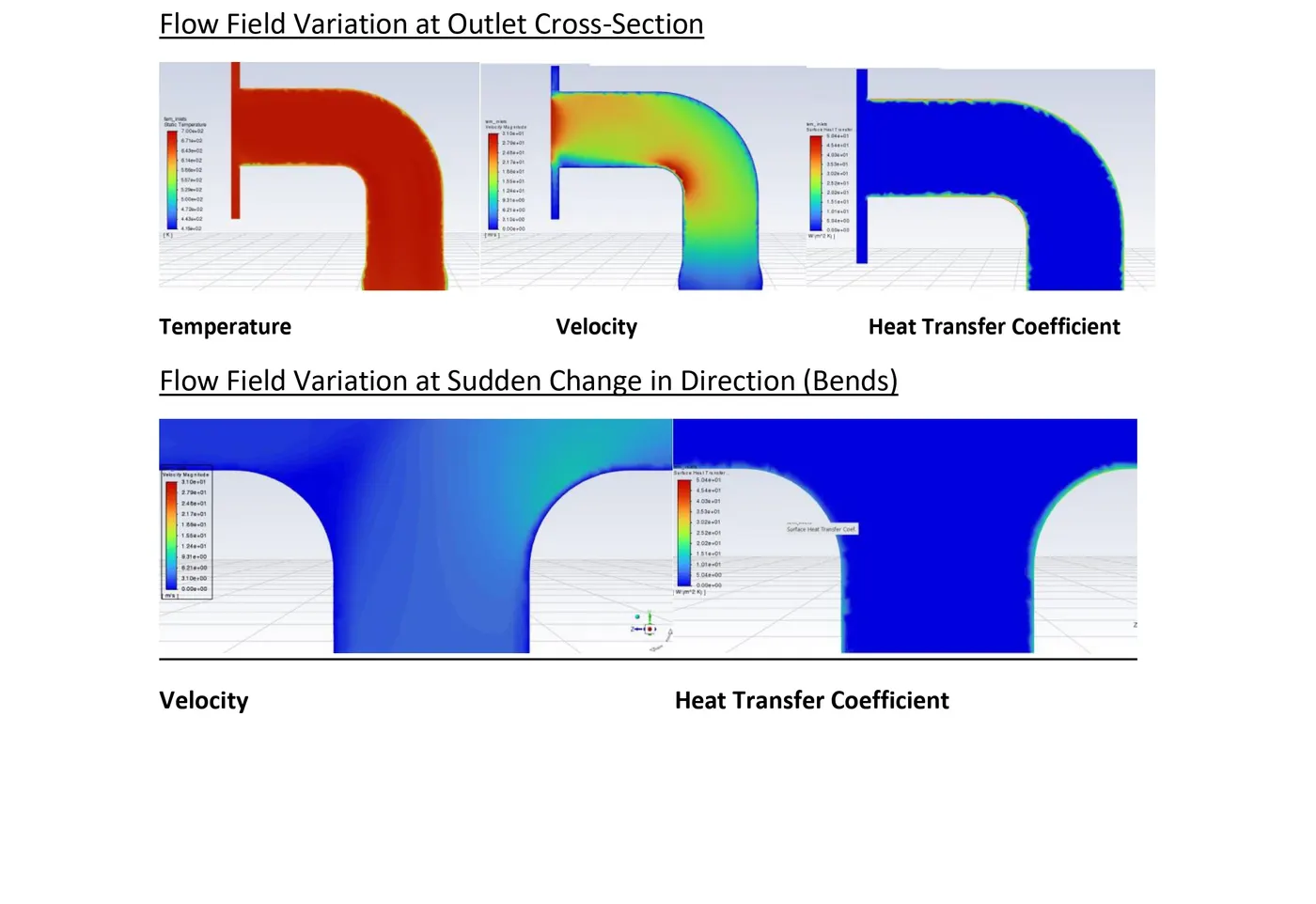
Figure 15: Flow Variables varying at outlet and other regions
At the bends if velocity increases due to decrease in pressure, the heat ttransfer coefficient also increases as it is directly dependent on flow velocity. This will increase the rate of heat transfer and greater amount of heat wil be expelled from these bending surfaces.
Step 6. Validation of Results
We can validate our results if our data is in close approximation to the one evaluated analytically.
First we check the value of surface heat transfer coefficient we ar getting then we will compare it to the one obtained from Dietus-Bolter Relation.
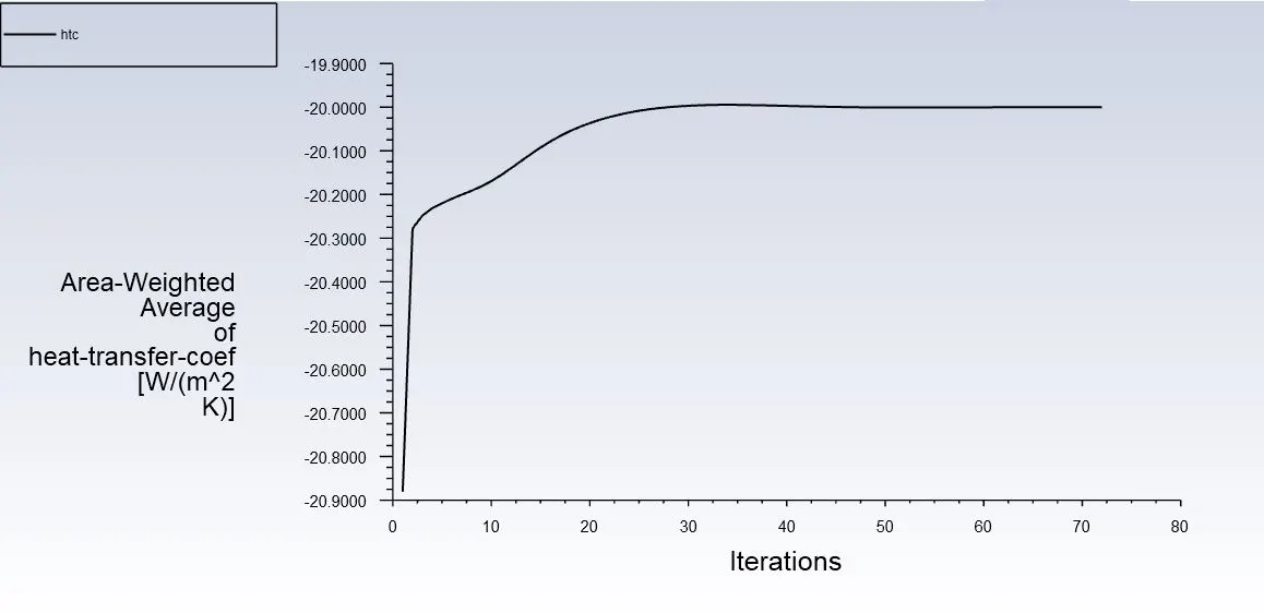
Surface Heat Transfer Coefficient = 20.000 W/m^2 K
Dittus-Bolter Relation
Nu(d) = 0.023*(Re)^4/5*(Pr)^n
Validity=> 0.6<=Pr<=160
Re,dh >= 10^4
L/d>10 [4]
n = 0.3*d = 0.3*0.166 = 0.0498
Pr = μ* Cp/K
μ = 1.789*10^-5 Pa s
Cp,air = 1006.43 j/kgK
K,air = 0.0242 w/mK
Pr =1.789*10^-5*1006.43/0.00242
Pr = 0.744
Nu(d) = 0.023*(Re)^4/5*(Pr)^n
= 0.023*(5.68*10^4)^4/5*(0.744)^0.0498
= 144.15
Nu = h*d/K
=> h = Nu*K/d
= 144.15*0.0242/ 0.166
= 21.015 W/m^2K
Calculated Value of surface heat transfer coefficient = 21.015 W/m^2K
Simulated Value of Surface Heat Transfer Coefficient = 20.00 W/m^2K
Since, our simulation is in close proximity of Empirical Measurements thus our results are validated.
Observations:
1. Conjugate heat transfer analysis is an effective tool to estimate heat transfer in devices where conduction and convection are both important.
2. Exhaust Manifold is critical device that works inline with the catalytic converter and plays a crucial role in emissions regulation.
3. In order to accurately measure surface heat transfer coefficient we need to capture the steep variation of the velocity profile near the wall that results in optimum Y+ value.
4. Meshing needs to be done with care, especially employing the inflation layers which leads to optimum y+ range.
5. Enhanced Wall treatment method being Y+ insensitive turned out to be the ideal choice. The range of y+ we obtained was 0.2<y+<200, thus where y+ was <=1, the near wall method was resolving the viscous-sublayer and where it was >30, it employed wall functions approach to capture the outer turbulent layer.
3. Selection of an approriate Turbulence Model with near wall effects was crucial in obtaining the accurate and converged results.
3. Our study found that the areas where velocity was higher, the surface heat transfer coefficient was also higher and rate of heat transfer was also higher.
4. Thus, by properly designing the exhaust manifold we can control the rate of heat transfer.
References
1. G. Mahadeven, S. Sendilvelan Temperature analysis of dynamic catalytic convertor system with pre-catalyst in a multi cylinder spark ignition engine to reduce light-off time. International Journal of Heat and Technology.
3. Fluid Mechanics, F. M. White