Week 4 - CHT Analysis on Exhaust port

CHT analysis for Exhaust Port

Aim

To verifying the exhaust port CHT analysis for through the Ansys software

Objective

•  brief description of why and where a CHT analysis is used.
• Maintain the y+ value according to the turbulence model and justify the results. 
•  wall/surface heat transfer coefficient on the internal solid surface & show the velocity & temperature contours in appropriate areas.
• verify if the HTC predictions and On what factors does the accuracy of the prediction .

Theory

Conjugate heat transfer analysis- Conjugate heat transfer analysis is based on the mathematical structure problem which describes the heat transfer between the body and the fluid flowing over or inside it as a result of interaction between two objects. At the matching interface, the details are provided for temperature distribution and heat flux along the interface eliminating the need of calculating the heat transfer coefficient.

CHT analysis type allows for the simulation of the heat transfer between the solid and liquid domains by exchanging thermal energy at the interface between them. The simulation of the heat exchangers, cooling of the electronic equipment, and general-purpose cooling and heating system.  In the case of CHT that is being done in this project, we have the convection mode of heat transfer between the fluid and the solid Aluminium wall of the exhaust pipe and then the conduction mode of heat transfer is followed within the wall of the exhaust pipe wall.

Solving and Modelling approach

 The exhaust pipe was model in the space claim.

2) The exhaust port is a three dimensional model containing four inlets and one outlet. Despite having the isothermal boundary condition and a uniform flow rate at the four inlets the model can not be cut into two halves to save computational power. Therefore the whole model needs to be discretized it is also called as space discretization.

3) CHT analysis requires the both the solid and the liquid volume under consideration spaceclaim gives an option of volume extract for selecting the edges for fluid volume.

4) Both the solid component and the liquid component are copied into one component.

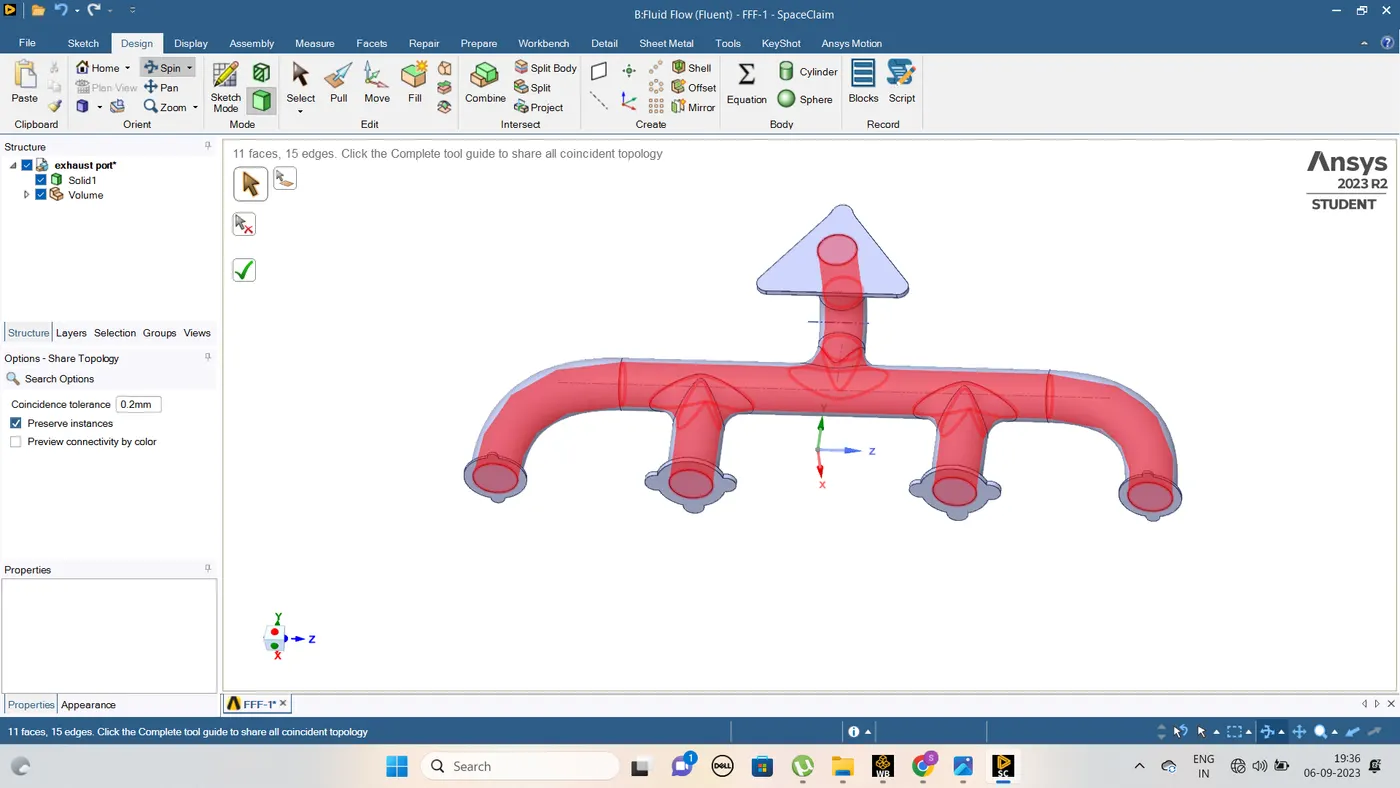
6) Spaceclaim gives an option for share coincident topology when share coincident topology is selected and executed. The mesh from the fluid volume and the solid volume are said to be conformal with each other which is a requirement for the CHT analysis.

In the model at present the extra edges and it should remove Repair-extra edges options through the removed.

Share topology is created.

Open mesh option check the cells count .

Create the inflation layer outer wall .This layer helps to surface heat transfer.

Mesh size will 20mm cells counts little bit high ,So we increasing the cells count due to body sizing meshing

Finally check the solution.

Geometry in Space claim option 

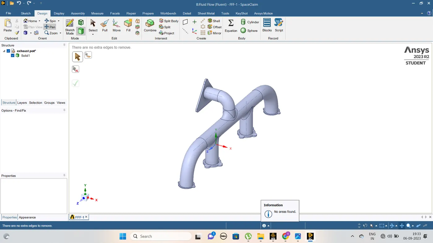
Insert the model through the spaceclaim.

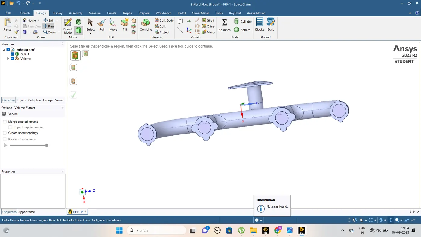
Then the volume extraction tool is used for the five edges and the volume and the process of fluid volume extraction is used for the edges to create the fluid volume.

Inside the spaceclaim the extra edges were found in the geometry that was provided we have to removed by the option of prepare and the six edges were removed.

finally the share the topology.

Mesh

Case 1

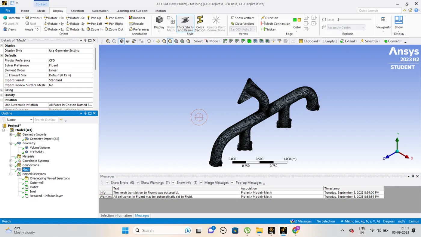
 Give the name selection inlet,outlet,outer wall.

The baseline mesh that is created due to the original geometry with less modifications-

Incraesing cell count reduce the mesh size

then creating the inflation layer 

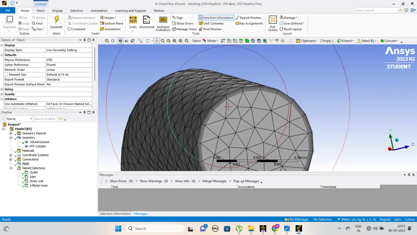
inflation layer added to the geometry in 5 layers

Growth ratio :1.2

number layers: 5

First layer thickness : 0.05

And then reduce the mesh size due to  body size meshing.

Setup

open the model

Double precision method

Solver processs give 4 the better solution

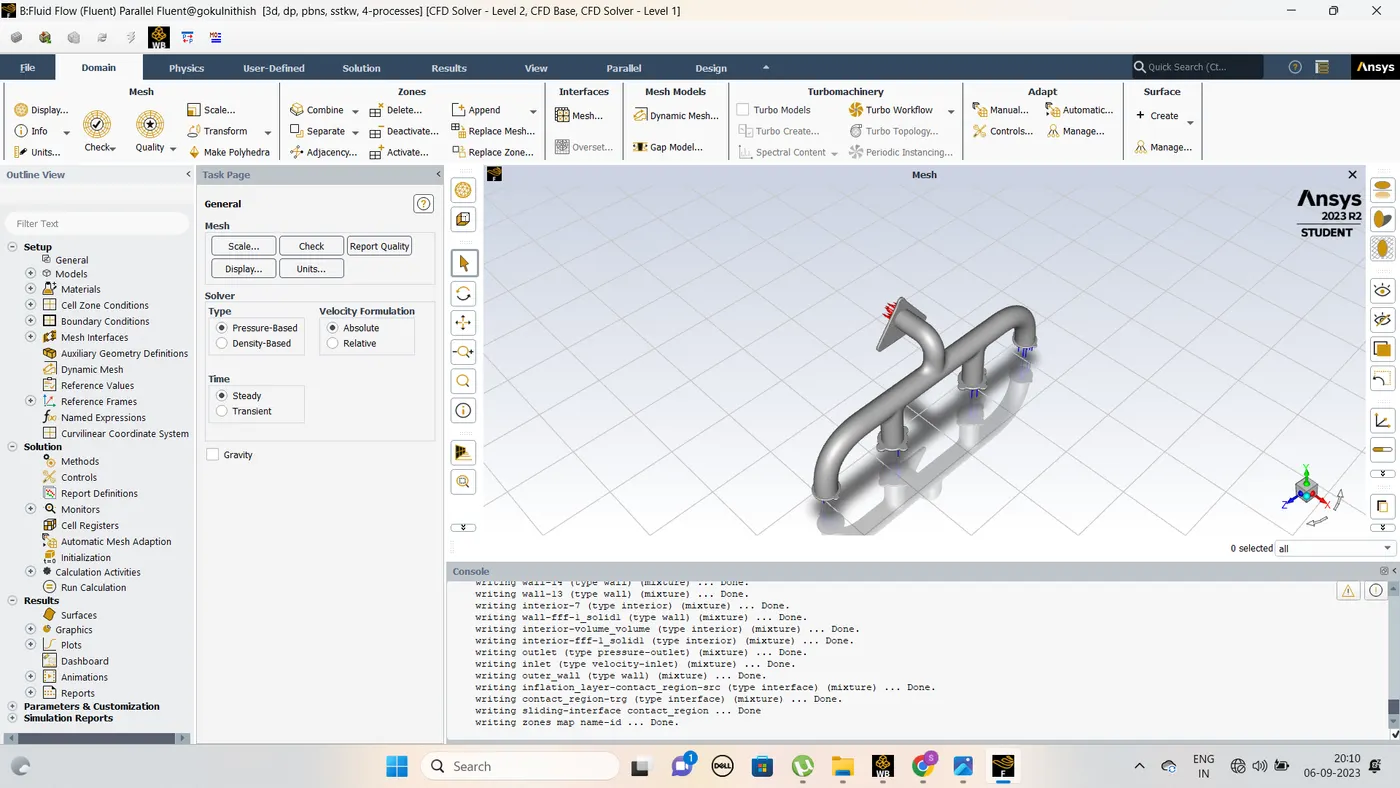
solver: Pressure based

Flow :Steady flow

Energy equation on

Material properties give to Solid model Aluminium as per aluminium value auto generate.

Boundries :Inlet -5m/s , Temperature =700k

Thermal conductivity =20 W/M-k

And the initialize the model.

Create  Velocity, Temperature contouure through the contour option.

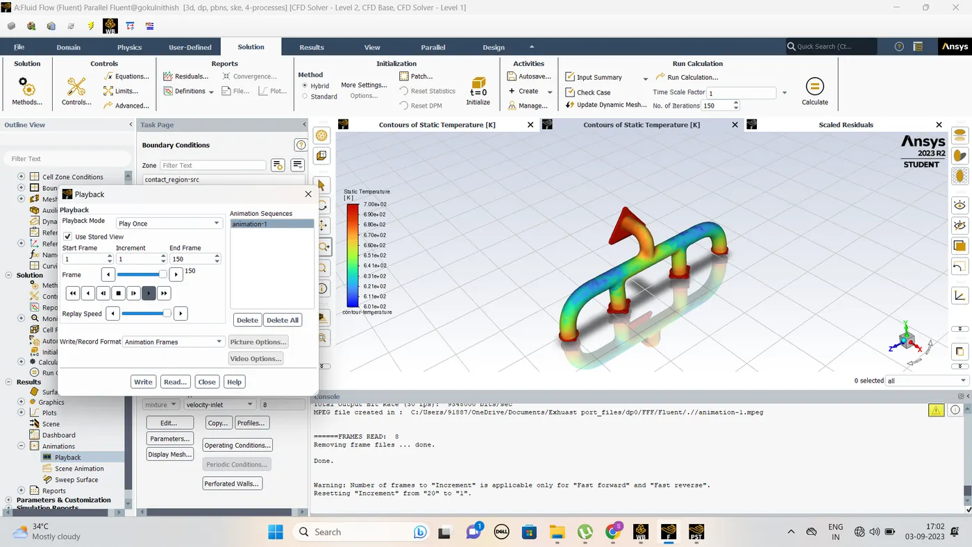
Create the animation then can show  visulize the heat transfer.

Finally iterate the model around the 150 iterations.

Showed the residual plot, Velocity and temperature contour .

Additionaly created Area Weightned avearage contours

Case 2

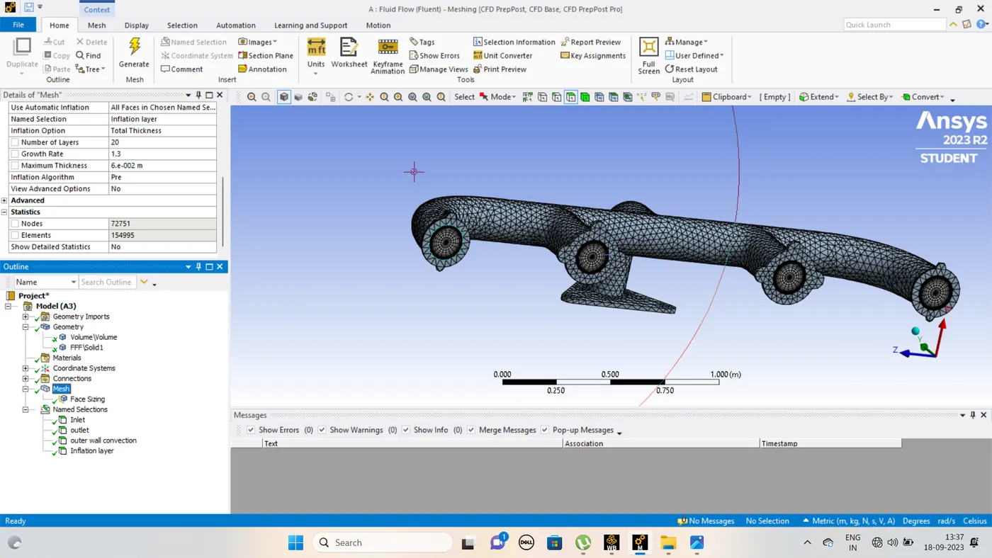
Mesh = 150 mm

Inflation layer

Growth ratio 1:3

First layer thickness 0.06

Inflation layer 

 

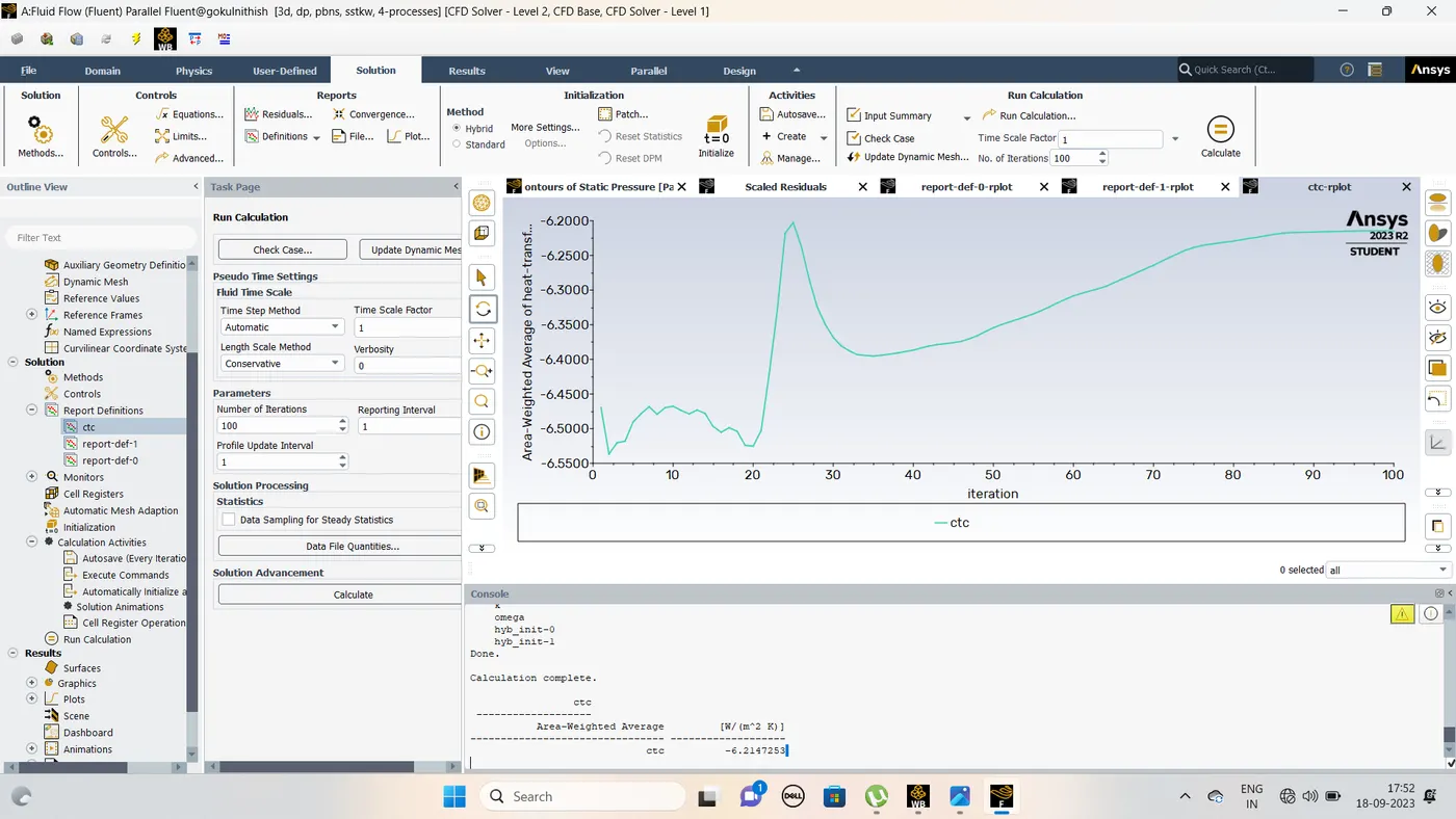
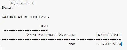
Temperature plot

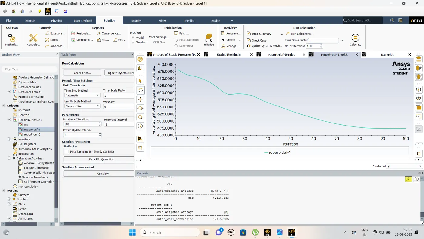
 Results are avearage temperature of outer wall convection 473.57K

Result

If setup the complete the model can the go result

Check the temperature, velocity  of the Exhaust port .

Double click - Colour - Variable - (Temperature and Velocity)- Apply

We know the Temperature proportional to the velocity.

Create the Streamline and the Velocity of lines.

Four inlet wall Flow the fluid flow one outlet wall.

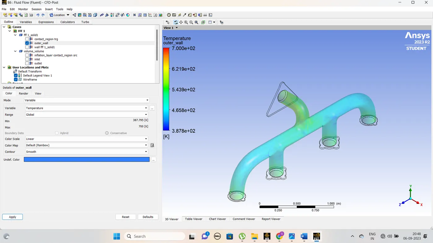
So velocity and Temperature will high of the outlet area

Streamline condition clearly Showed  the outlet.Outlet area velocity very high.

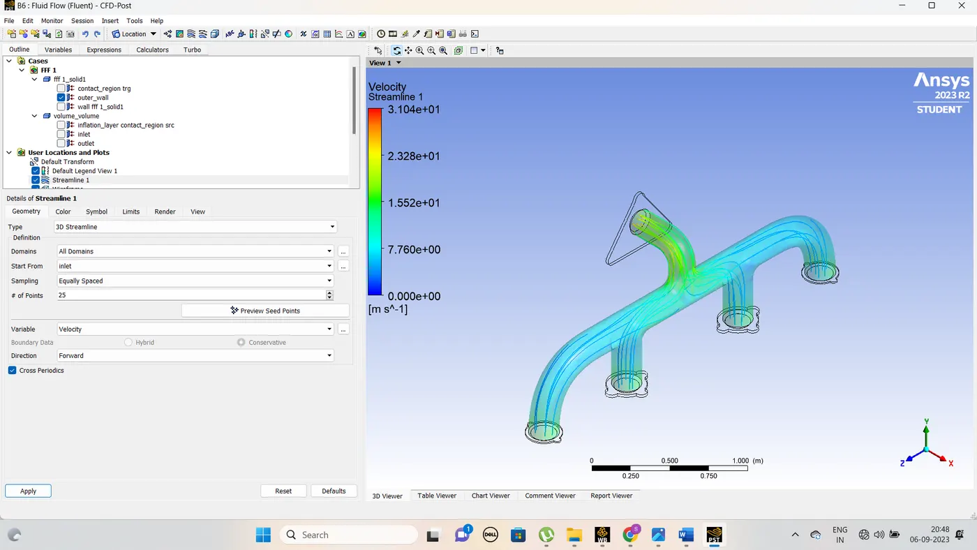
Plane 1

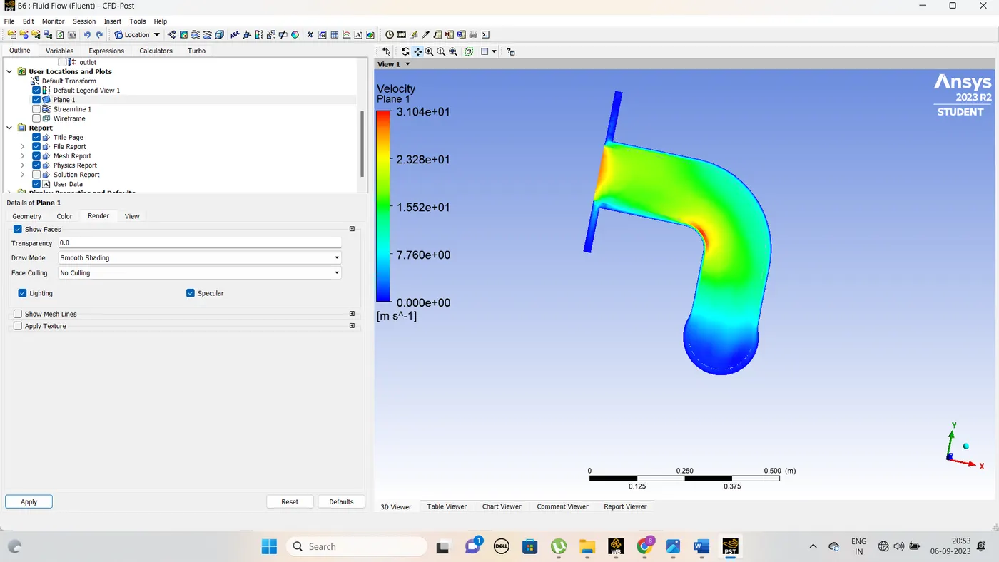
 Create a plane XY dxn,Variable give velocity near outlet of the contour

above image detail showed outlet of valve is the high velocity flow occured.

Valve bend Side also high velocity threre.

If high velocity there also temperature also high.

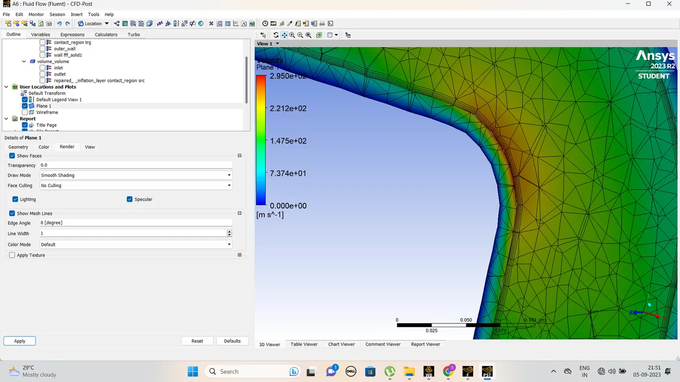
Above Snaps are clearly showed inflation layer show the near wall heat transfer

Inflation layer clearly showed Surface heat transfer coeficient.

Finally fining mesh show the heat transfer of the wall.

How would you verify if the HTC predictions from the simulations are right? On what factors does the accuracy of the prediction depend on?

The typical flow conditions in automotive exhaust systems produce Re numbers in the range of 10^3 to 5*10^4 . The exhaust flow often enters the region Re< 2300>

According to the Sieder Tate relation which correlates the Nu number with Re and Pr

It means Nusselt no. is the function of Reynolds no. and Prandtl no.

As the turbulent boundary layer in the vicinity of bend at outlet port is thin maximum velocity of flow is observed at bend and hence higher Reynold no.

Now, Nu = h*L/K

As Length of pipe and thermal conductivity are constant, value of h will increases as Nu increases and Nu increases as Re increases.

As per our results, heat transfer coefficient is high for higher value of velocity and hence from above discussion we think that our result .