Week 4 - CHT Analysis on Exhaust port
CHT is an analysis or simulation of heat transfer phenomena where Conduction and Convection takes place simultaneously. It is typically used for studying heat transfer between Solid surfaces like wall and surrounding fluid elements like air, oil etc.
This type of analysis is used, where heat transfer play major role. Some of the fields are Aerospace, Automotive, Power Generation, Electronic cooling etc.
For the Exhaust port we will run 3 cases
1st Case: Baseline Mesh
2nd Case: Refined Mesh with y+ = 1
3rd Case: Refined Mesh with y+ = 1
Pre-Processing:
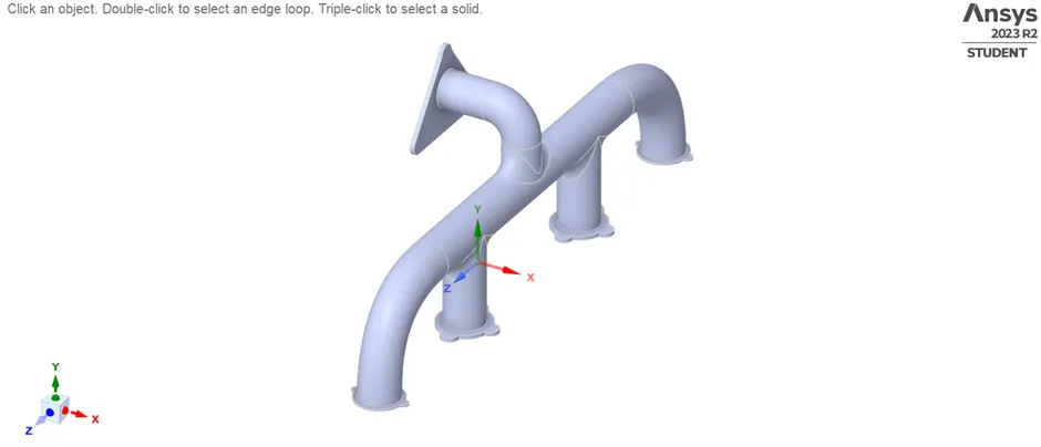
1) We will first import the model in Spaceclaim
<!--[endif]-->
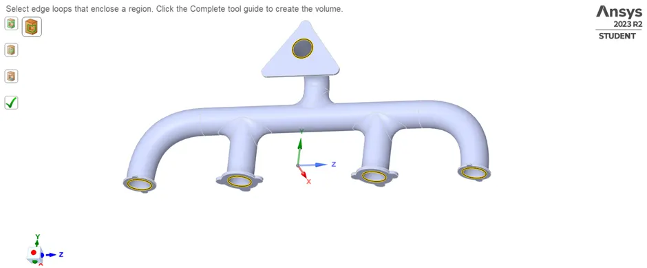
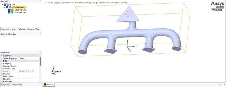
2) Now we will extract fluid volume using edge selection.
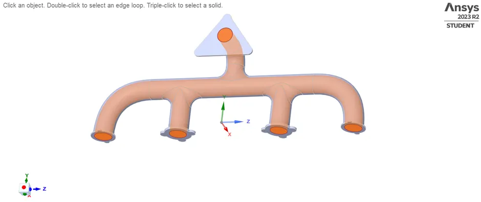
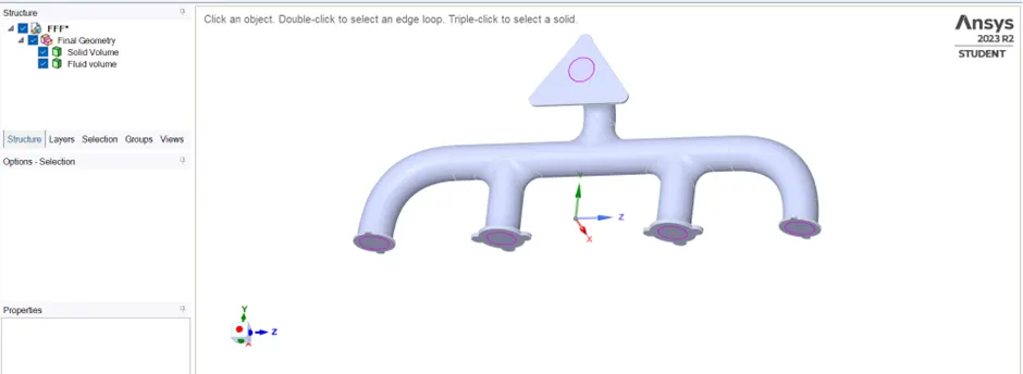
3) Now we need to move both the solids under new component as Final Geometry.
<!--[endif]-->
4) Then we need to share topology between solid and fluid for proper mesh arrangement between the two solids.
1st Case:
a) Meshing:
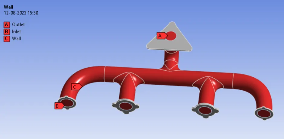
1) Once we open Meshing, we have to create named selections
<!--[endif]-->
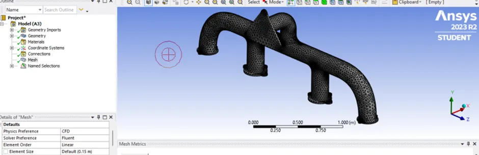
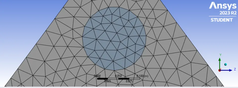
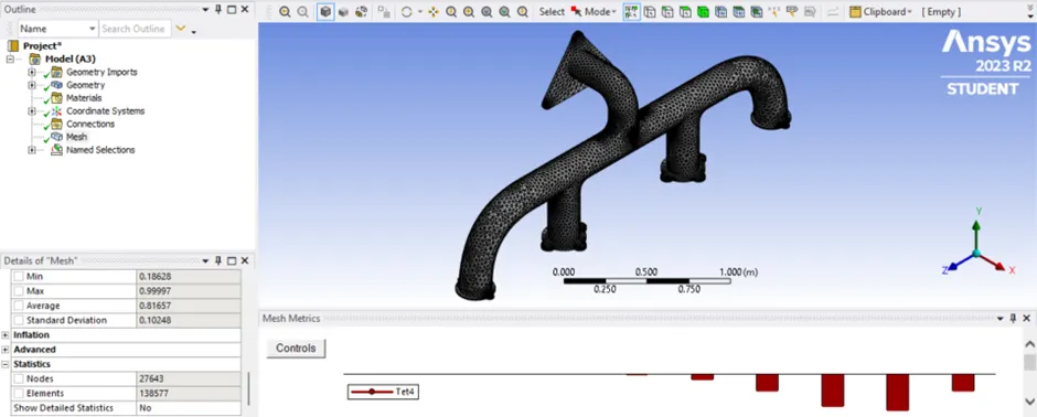
2) We will perform a default meshing for the exhaust port just get the feel of the solution.
<!--[endif]-->
<!--[endif]-->
3) Mesh elements and Quality Statistics
<!--[endif]-->
b) Solving:
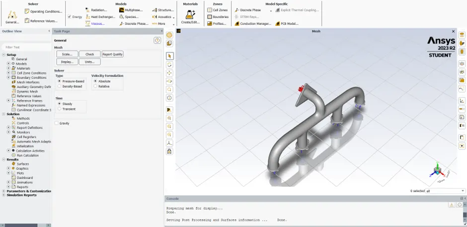
1) Now we will open fluid flow fluent to setup Boundary Condition
<!--[endif]-->
<!--[endif]-->
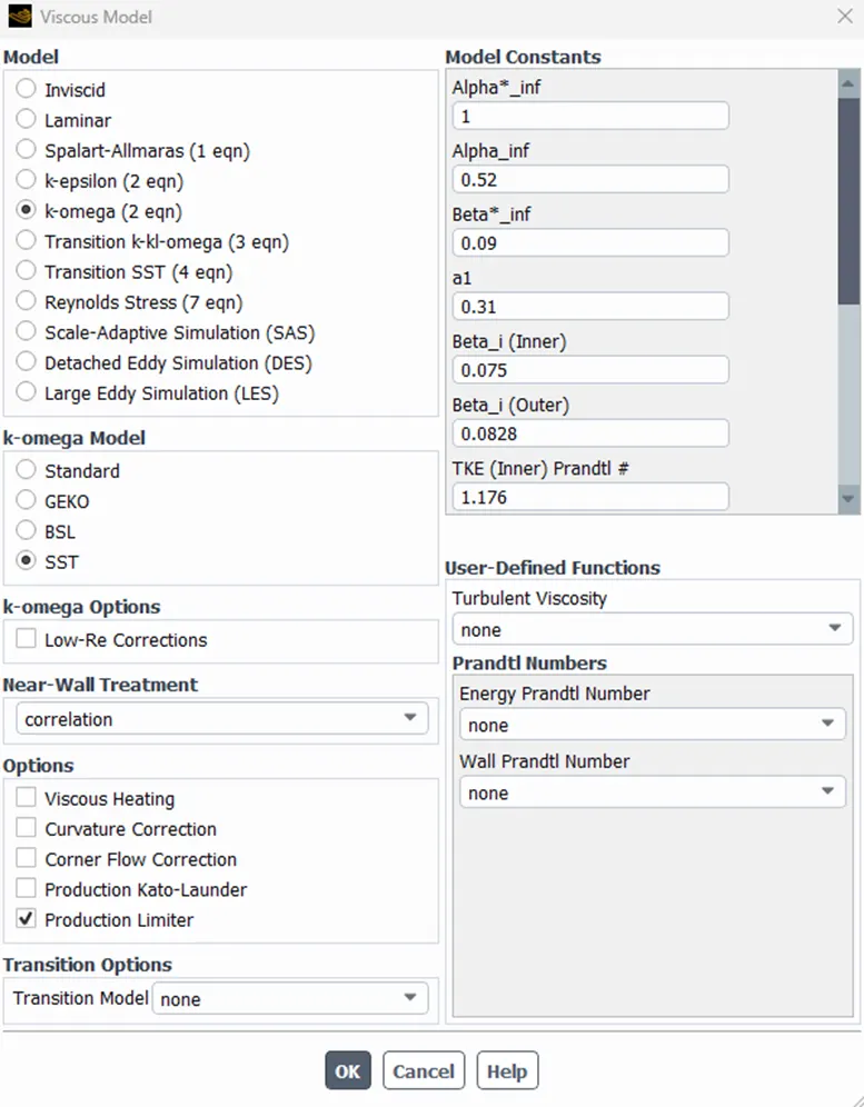
We will use K-omega turbulence model here as it gives more accurate results near wall
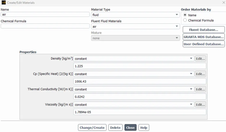
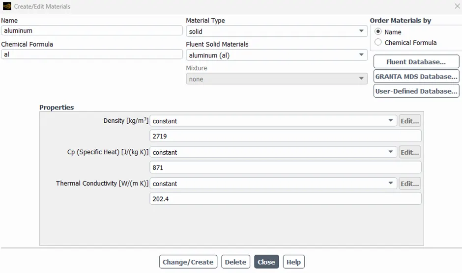
2) Materials for fluid and solid are as follows:
<!--[endif]-->
<!--[endif]-->
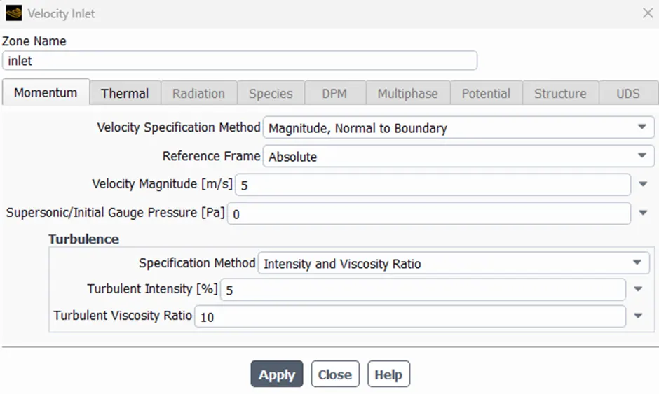
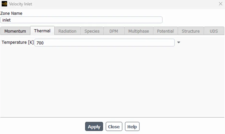
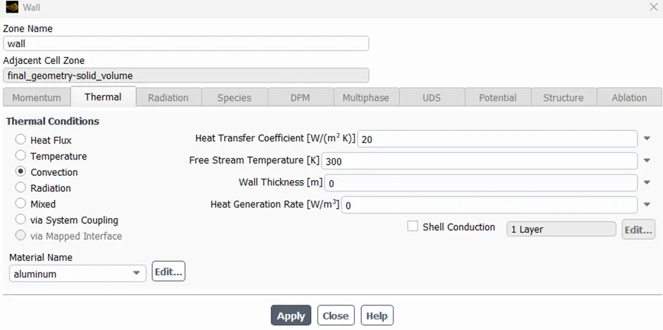
3) Boundary condition for inlet, wall and outlet
Inlet
<!--[endif]-->
<!--[endif]-->
Wall
<!--[endif]-->
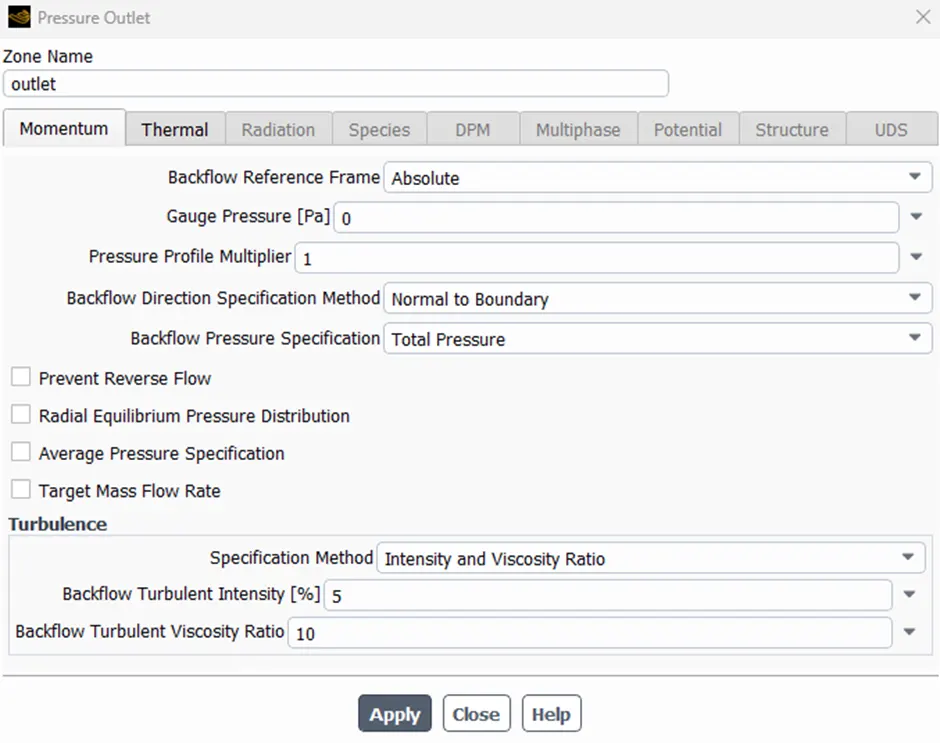
Outlet
<!--[endif]-->
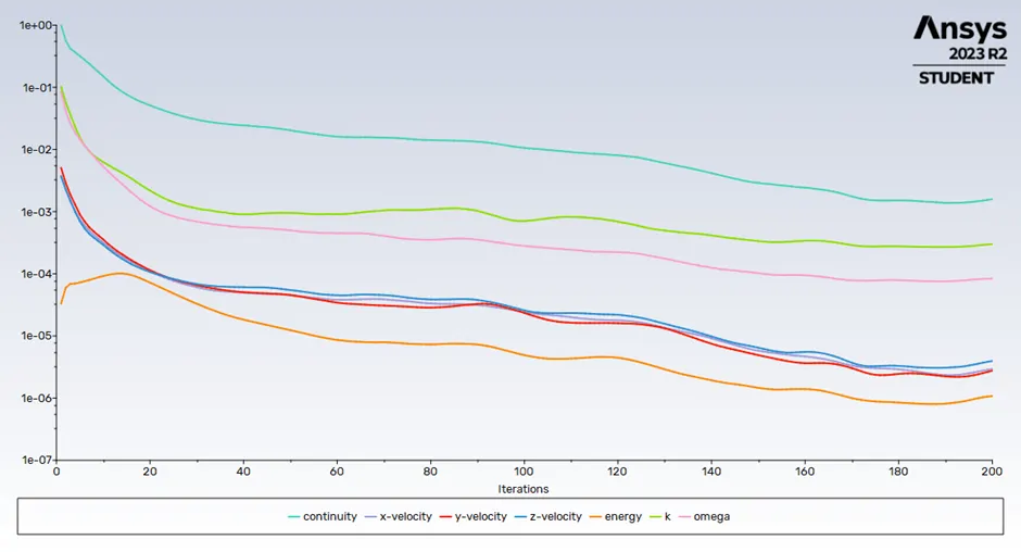
4) After running simulation for 200 iterations the solution seems converged. Residual chart as below
<!--[endif]-->
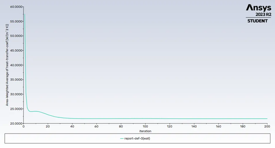
5) Heat Transfer Coefficient Chart:
<!--[endif]-->
We got a net heat transfer coefficient of 21.6168 W/m^2 K
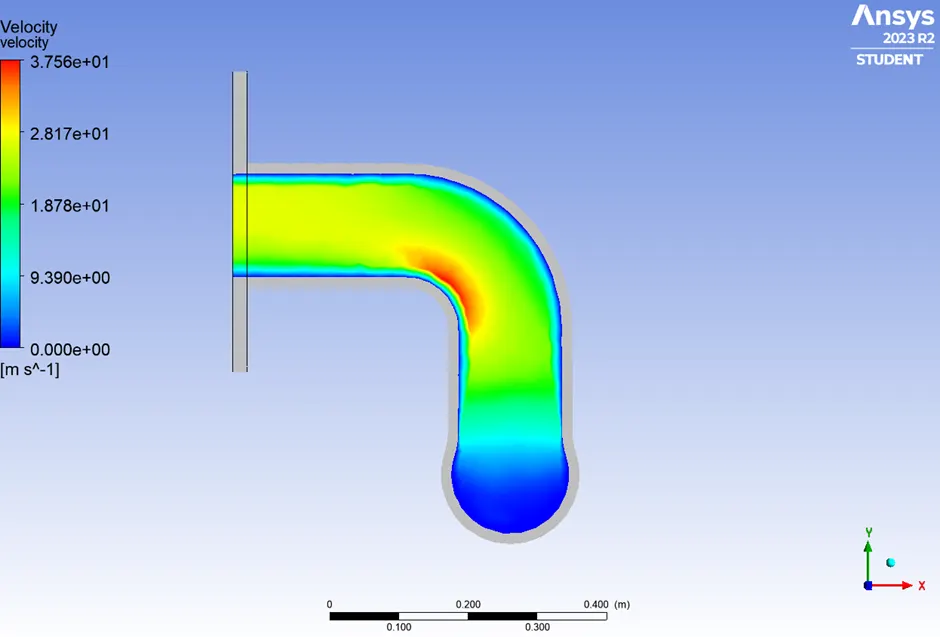
6) Velocity Plot:
<!--[endif]-->
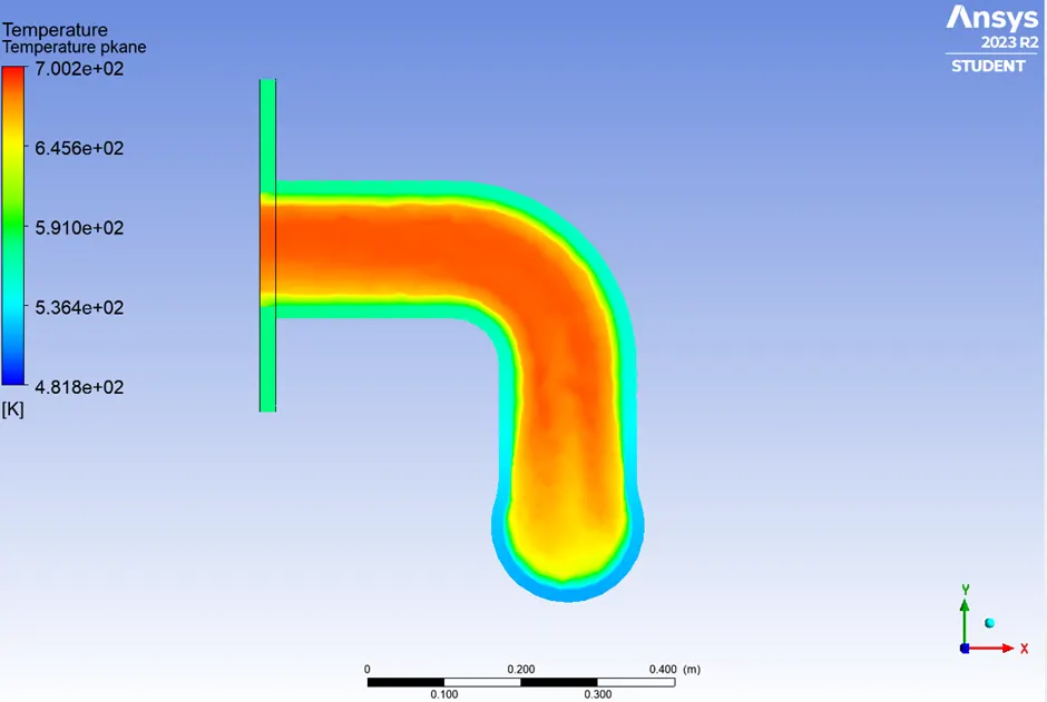
7) Temperature Plot:
<!--[endif]-->
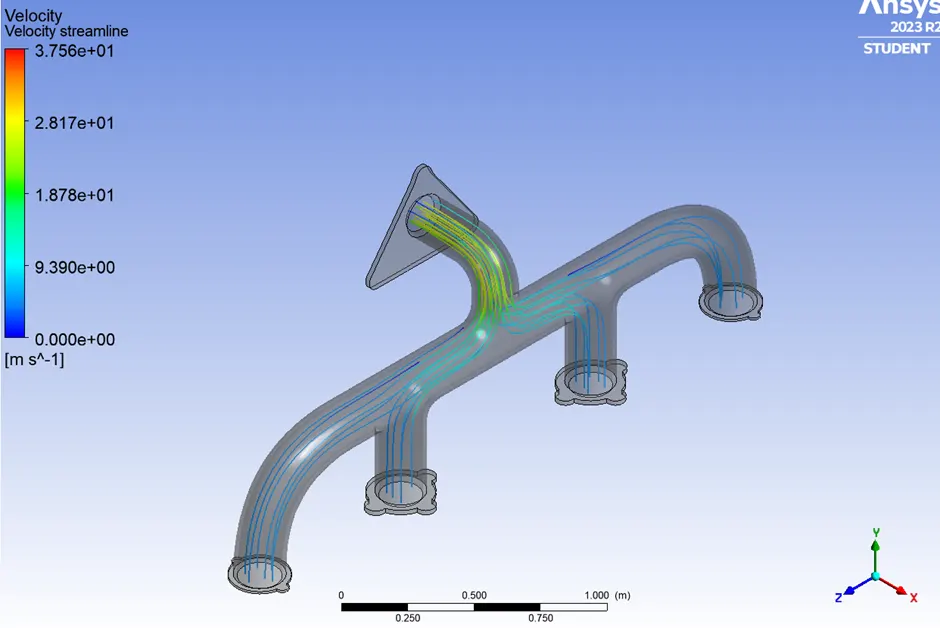
8) Velocity Streamline:
<!--[endif]-->
2nd Case:
a) Meshing:
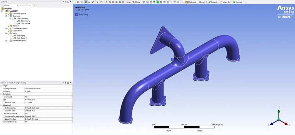
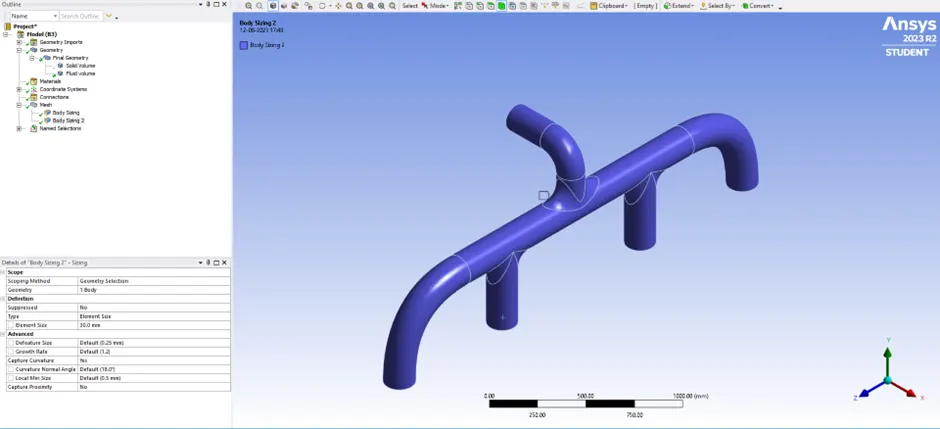
1) We will now refine the mesh. We will keep 50 mm for the solid body and 20 mm to fluid body
<!--[endif]-->
<!--[endif]-->
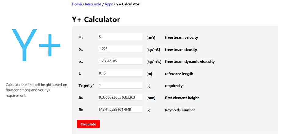
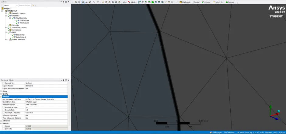
2) We will also add inflation layer considering y+ value as 1
<!--[endif]-->
So, the first layer thickness will be 0.05560 mm and number of layers will be 10. So, total thickness will be 0.5560 mm
<!--[endif]-->
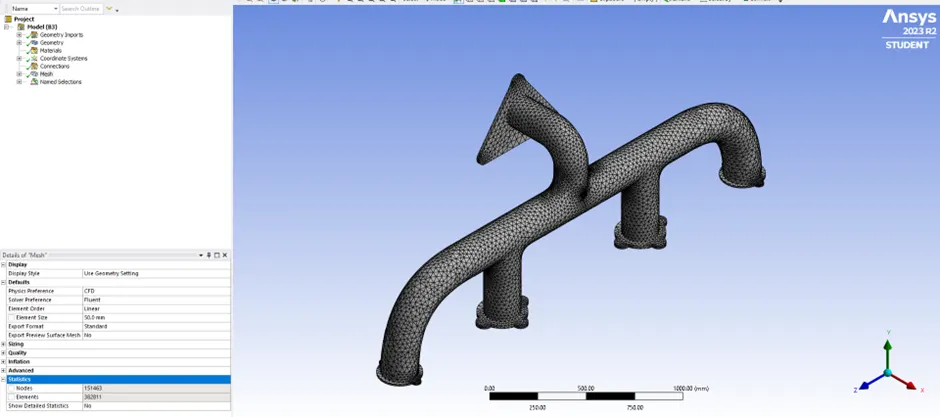
3) Mesh elements statistics:
<!--[endif]-->
b) Solving:
1) Boundary condition will remain same as in the case 1.
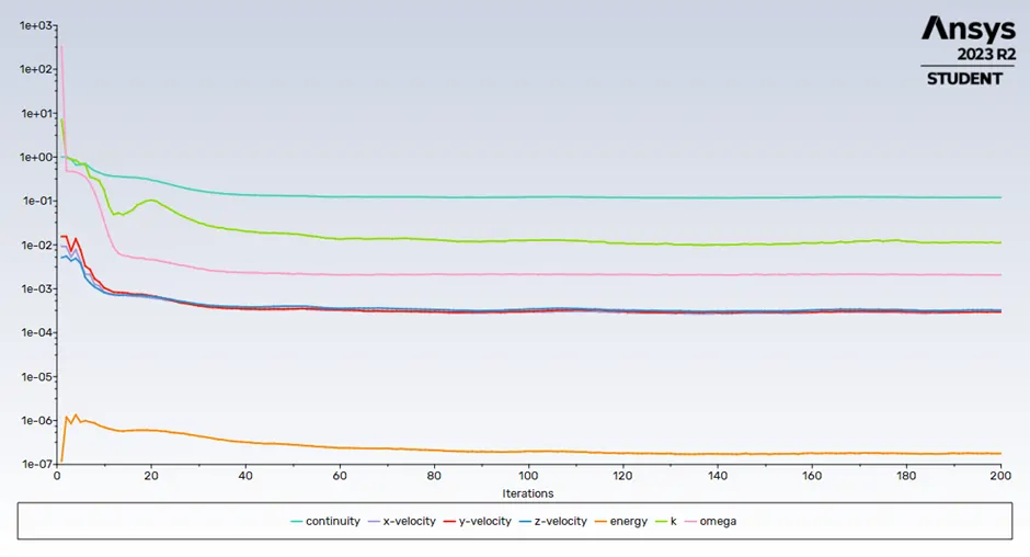
2) Residual chart:
<!--[endif]-->
3) Heat Transfer Coefficient Chart:
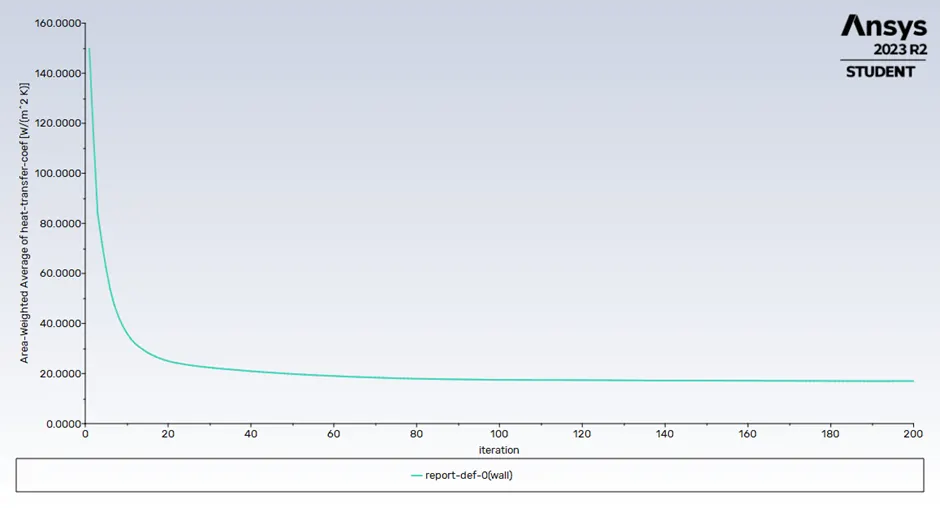
We got a net heat transfer coefficient of 16.9951 W/m^2 K.
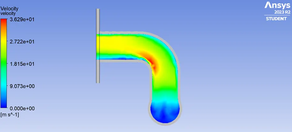
4) Velocity Plot:
<!--[endif]-->
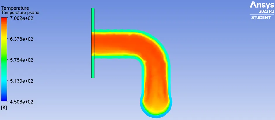
5) Temperature Plot:
<!--[endif]-->
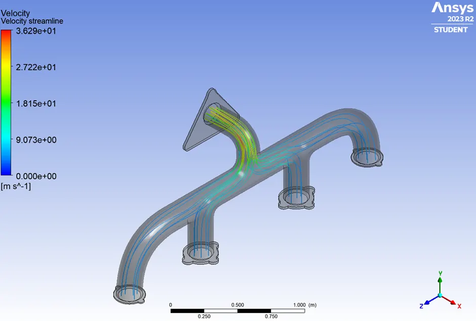
6) Velocity Streamline:
<!--[endif]-->
3rd Case:
a) Meshing:
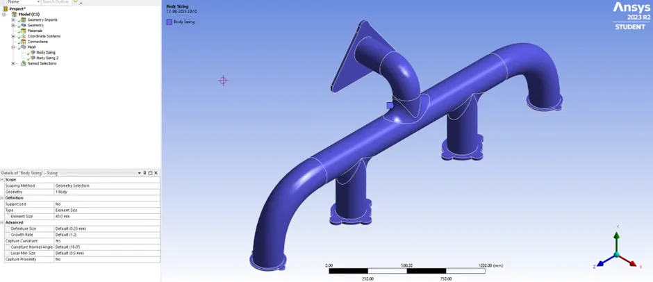
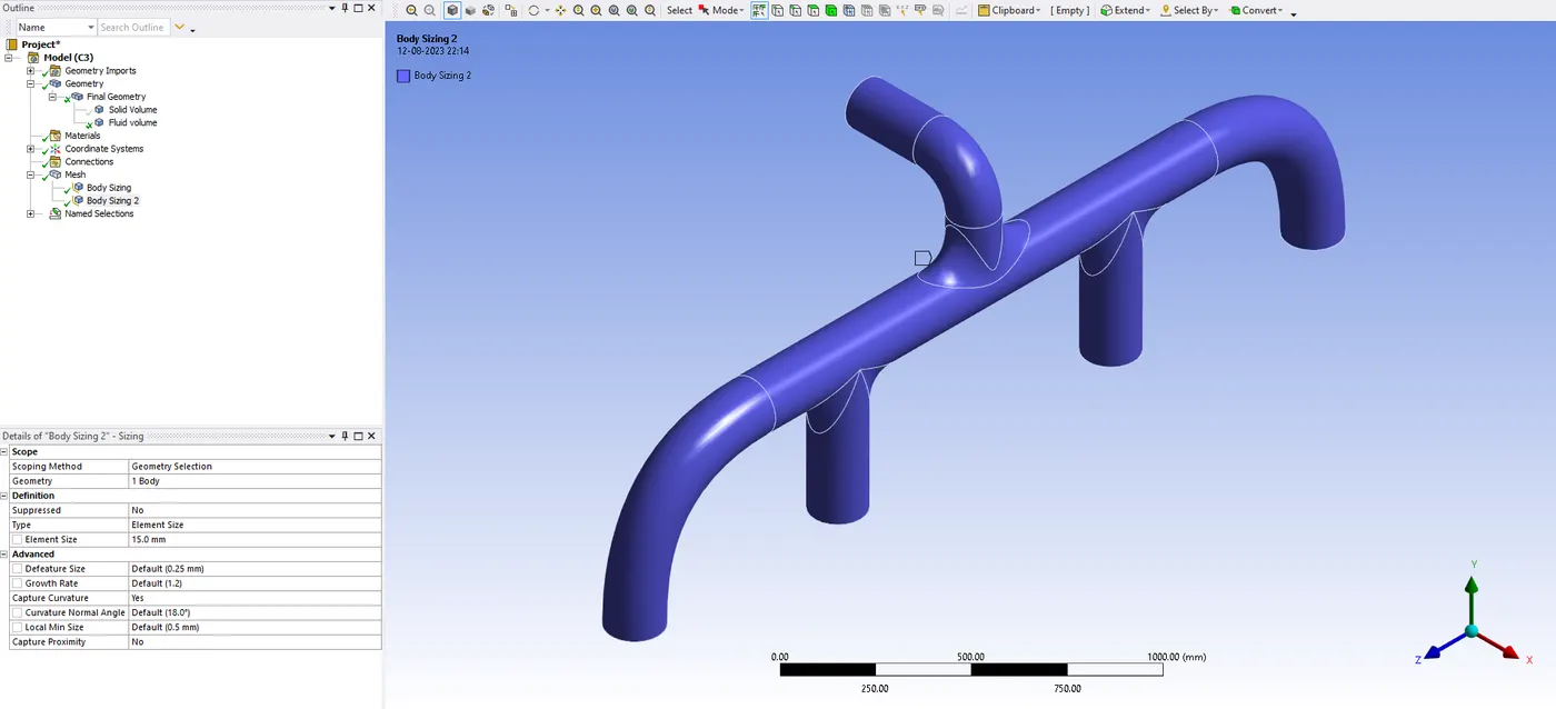
1) We will now refine the mesh. We will keep 40 mm for the solid body and 15 mm to fluid body
<!--[endif]-->
<!--[endif]-->
2) We will also add inflation layer considering y+ value as 1
<!--[endif]-->
So, the first layer thickness will be 0.05560 mm and number of layers will be 10. So, total thickness will be 0.5560 mm
<!--[endif]-->
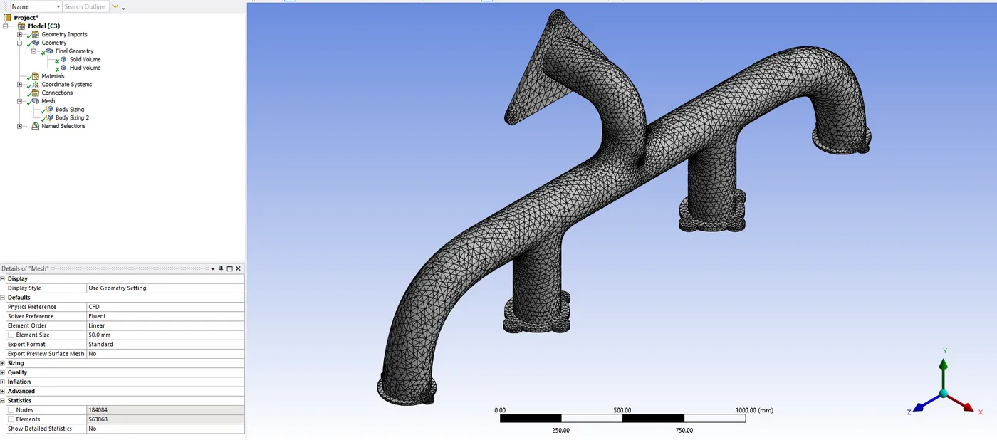
3) Mesh elements statistics:
<!--[endif]-->
b) Solving:
1) Boundary condition will remain same as in the case 1.
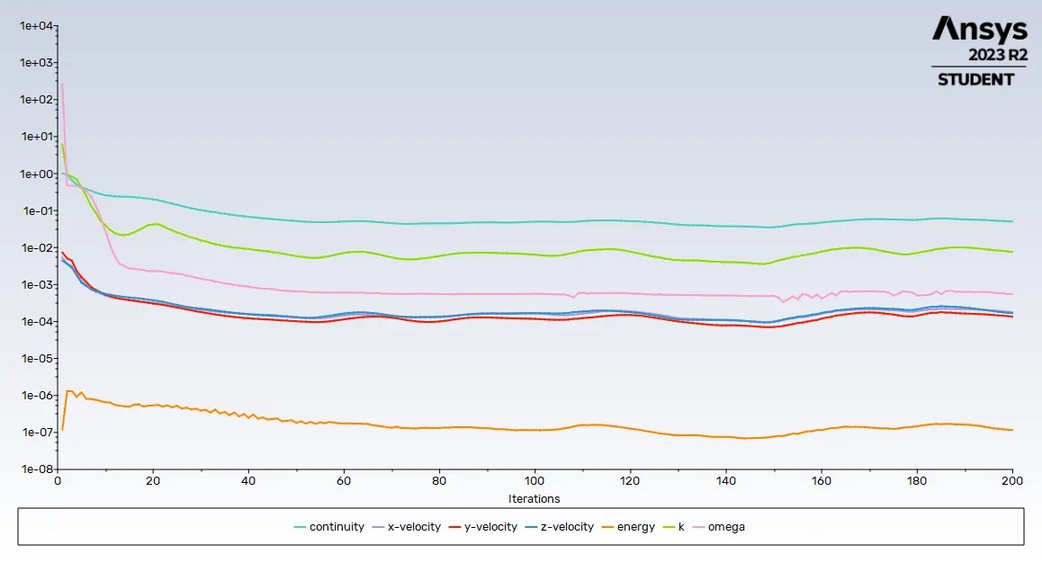
2) Residual chart:
<!--[endif]-->
3) Heat Transfer Coefficient Chart:
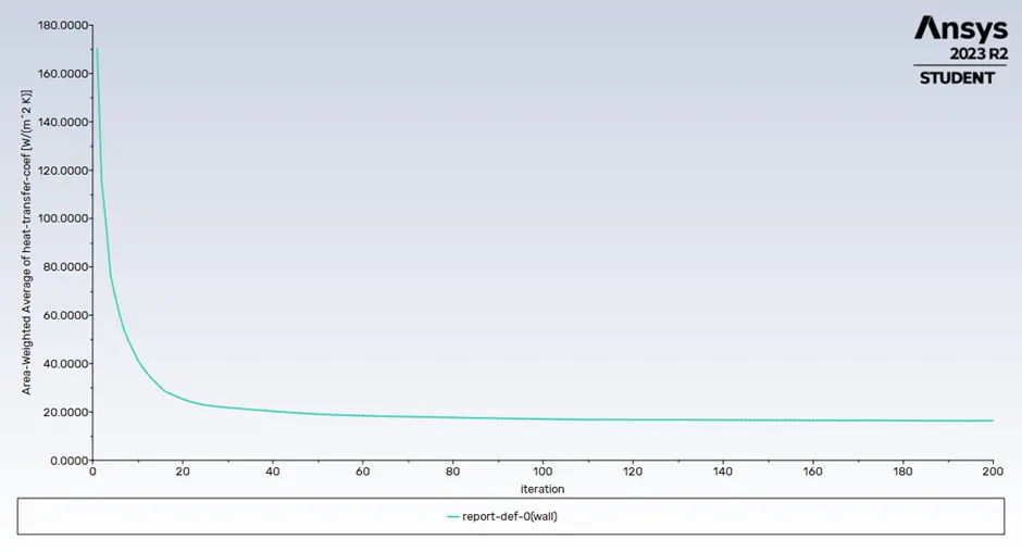
We got a net heat transfer coefficient of 16.39 W/m^2 K.
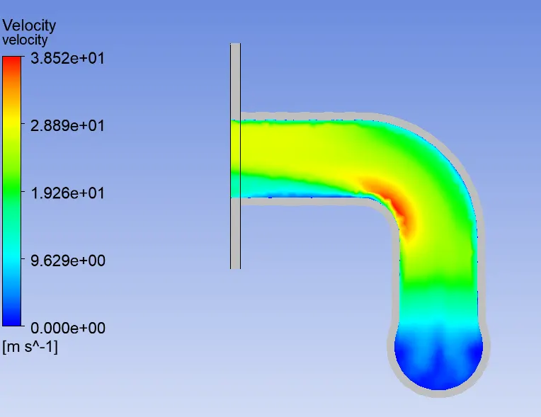
4) Velocity Plot:
<!--[endif]-->
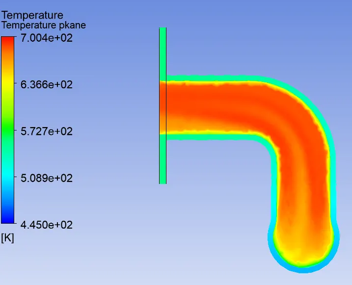
5) Temperature Plot:
<!--[endif]-->
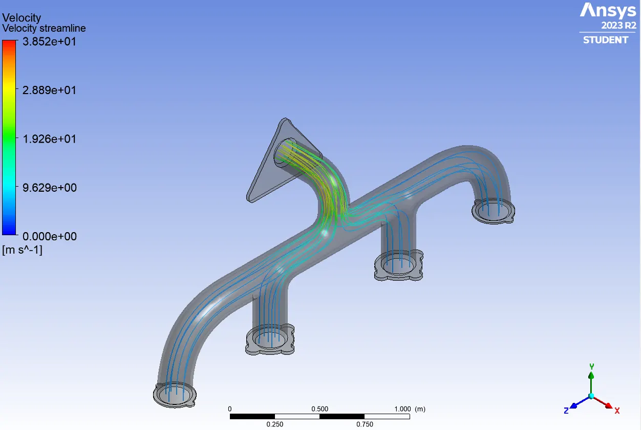
6) Velocity Streamline:
<!--[endif]-->
Analytical Solution:
Pr = μ * Cp/K
where μ = Dynamic Viscosity = 1.7894e-05 Pa·s
Cp = Specific heat capacity = 1006.43 J/(kg·K)
K = Thermal conductivity = 0.0242 W/(m·K)
So, by substituting above value in the equation we get
Pr = 0.744
So, we will now substitute Pr and Re (i.e., 51344.025) in Nusselt number equation shown in above image.
Nu = 0.023*(Re^0.8)*(Pr^0.4)
Nu = 119.88
For Nusselt number we have another formula i.e,
Nu = h*L/K
where h = heat transfer coefficient
L = characteristic length = 0.15 m
K = Thermal conductivity = 0.0242 W/(m·K)
So, for h we can write eqaution as
h = Nu*K/L
And substituting above values in the eqaution we get
h = 19.34 W/(m⊃2;·K)
Comparison:
| Sr No. | Mesh Size (in m) | Analytical Solution for h (in W/(m⊃2;·K)) | Numerical Solution for h (in W/(m⊃2;·K)) |
| 1 | 0.15 - S&F | 19.34 | 21.6168 |
| 2 | 0.05 - S, 0.02 - F | 16.9951 | |
| 3 | 0.04 - S , 0.015 - F | 16.39 |
Where S represents Solid body and F represents Fluid Body
Conclusion:
1) We performed the mesh independency test, and we can conclude that as the mesh is being refined the value for h is almost same.
2) If we compare between analytical solution and numerical solution we see that there is a difference and with more refinement the solution will not be similar to the analytical solution. So, I conclude that some assumption made during analysis might be wrong.