Week 4 - CHT Analysis on Exhaust port

Conjugate Heat Transfer:-

Conjugate Heat Transfer analysis describes the heat transfer between the solid body and the fluid flow inside the soild or over the solid body in a mathematical form, that requires the temperature distribution and rate of heat flux at the interface and that results to calculates heat transfer coefficient.

Basically CHT (Conjugate Heat Transfer analysis) is a type of stimulations of heat transfer between the solid and fluid surfaces. Here the way of heat convection analysis takes place between the solid and fluids. This type of analysis is mainly used in stimulation of components like heat exchangers, electronic components, the exhaust parts of engines, and engine fins and so on.

CHT analysis on Exhaust port:

• Open the splace claim and load the geomentry.
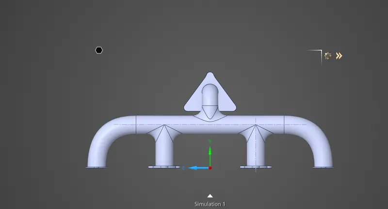
• Here, we observe there are four inlet and one outlet port, there the exhaust gases are coming from four inlets and then passes throught the one outlet, so we assume that the outlet port has more temperature of gases compare to the inlet gas temperature and also assume that air outside the model as specific heat transfer coefficient and Reynolds number that taken as input to out stimulation.
• So, first we need to extract the inside flow volume on the model using volume Extract tool and select the edges of the opening ports. After that splaceclaim need to consider the both the volumes i.e..., the splid and fluid volumes into one common volume, so create a new geometry called final geomentry by combining the two volumes.
• After, that to share the topological information between the two volumes create the share topology.
  
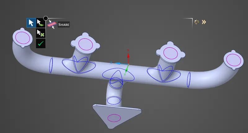
• Now move on to meshing part, so give the named selections to the loaded geomentry as inlet, outlet and outer-wall-convecton, and the rest of the surfaces have the adiabatic condition so heat transfer not takes place those surfaces.
  
  CASE 1:-
• And if we mesh the baseline model with default setup the mesh is not that much refined to stimulate and the no.of elements formed are 171702, and the mesh look like this form.
  
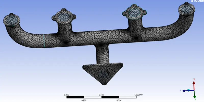
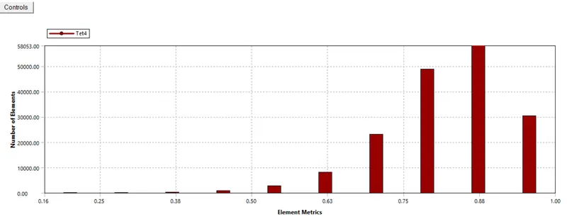
• And the mesh metric quality of the model is as shown below with 171702 number of elements and 33554 number of Nodes, and also the element metrics quality is in between 0.16 - 1.00 
  
• After that import the meshed baseline model to the Fluent solver and setup the stimulation conditions.
• Setup the viscous model to k-epsilon and able the energy equation.
• And take fluid material as air and soild material as aluminium.
• Material Properties:
  Fluent fluid material: Air
  Density: 1.225kg/m^3
  Specific heat: 1006.43 j/kg.k
  thermal conductivity: 0.0242 W/m.k
  Viscosity: 1.7894e-05 kg/m.s
  
  Solid Fluent material: Aluminium (al)
  Density: 2719 kg/m^3
  Specific heat: 871 j/kg.k
  thermal conductivity: 202.4 W/m.k
• Boundary conditions:
  Inlet: 
  Inlet type: velocity-inlet
  Velocity: 5 m/s 
  Temperature: 700k
  outer-wall-convection:
  heat transfer coefficient: 20 w/(m^2.k)
  outlet:
  outlet type: pressure -outlet
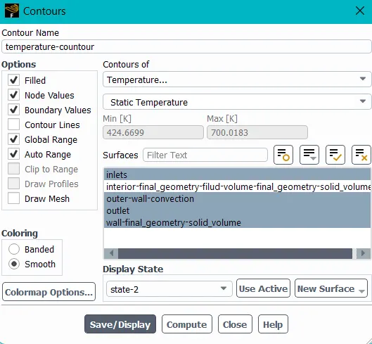
  Gauge pressure: 0
• After that create a temperature contour on the inlet, outlet, outlet-wall-convection, final-wall-geomentry.
  
• Then initialize the stimulation of 150 iterations and observe the results.
  Residuals: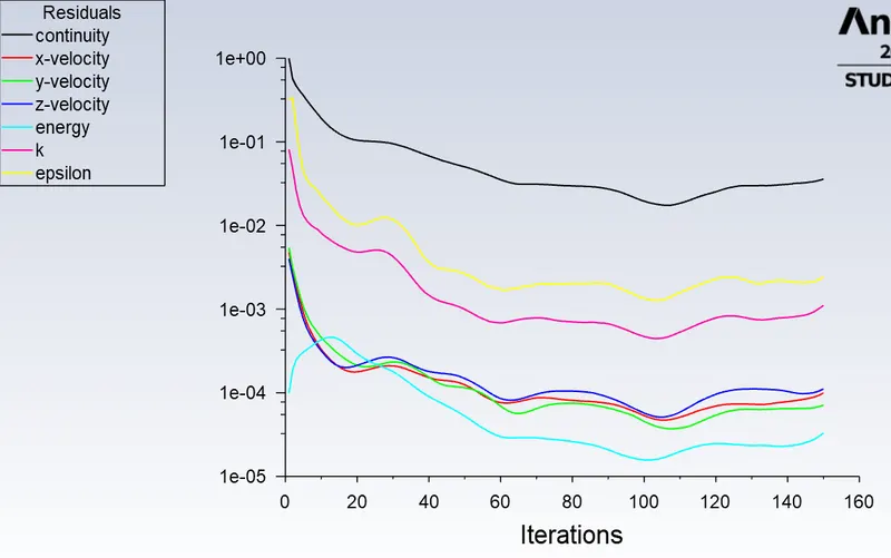
  
  heat transfers coefficient: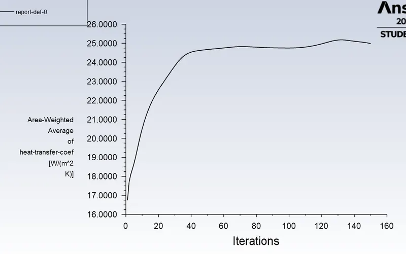
  
• And the Area-Weighted Average of heat transfers coefficient is 24.988108 W/(m^2 K).
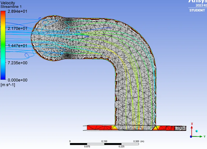
• The steemline flow of velocity 
  
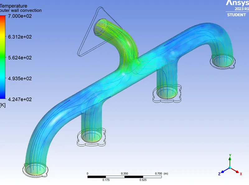
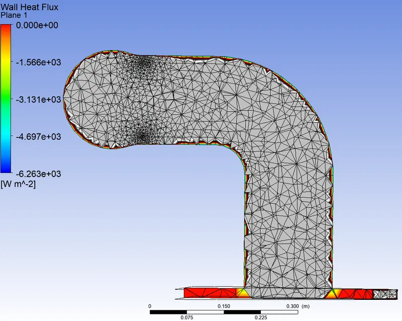
• And the wall heat flux
   
• And the velocity steamline 
  
  
  
  
  CASE 2:-
• In this case refine the model by applying an inflation layer and refining the soild geometry to a refined element size.
  The inflation object is set to Total Thickness
  Growth rate is 1.2 mm
  Maximum Thickness 6mm
• And turn on the Capture cirves default setup.
• And the refined mesh is looks like as below
  
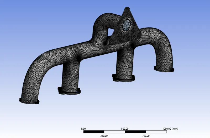
• And the number of elements for the refined model are 404529, and the number of elements are 123798.
• And apply the same solver setup to the refined model and the results are mentioned below
  Residuals: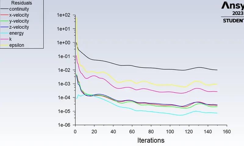
  
  Temperature contour: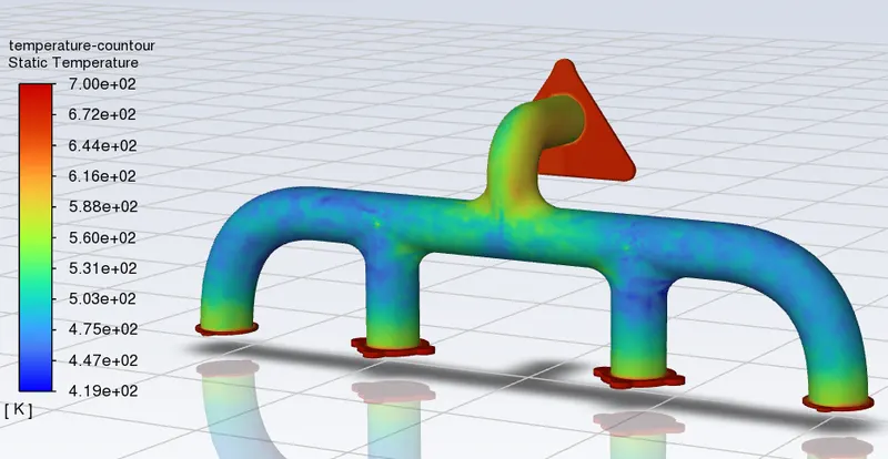
  
  heat transfers coefficient: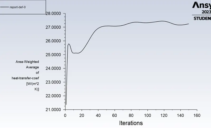
  
  
  
• And the Area-Weighted Average of heat transfers coefficient is 27.241283 W/(m^2 K).
• The steemline flow of velocity 
  
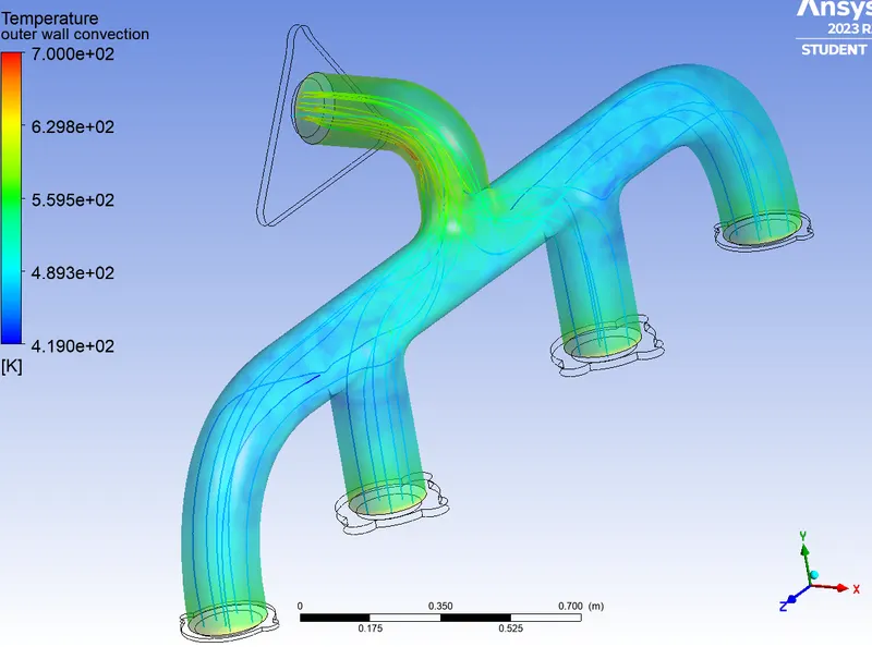
• And the wall heat flux
  
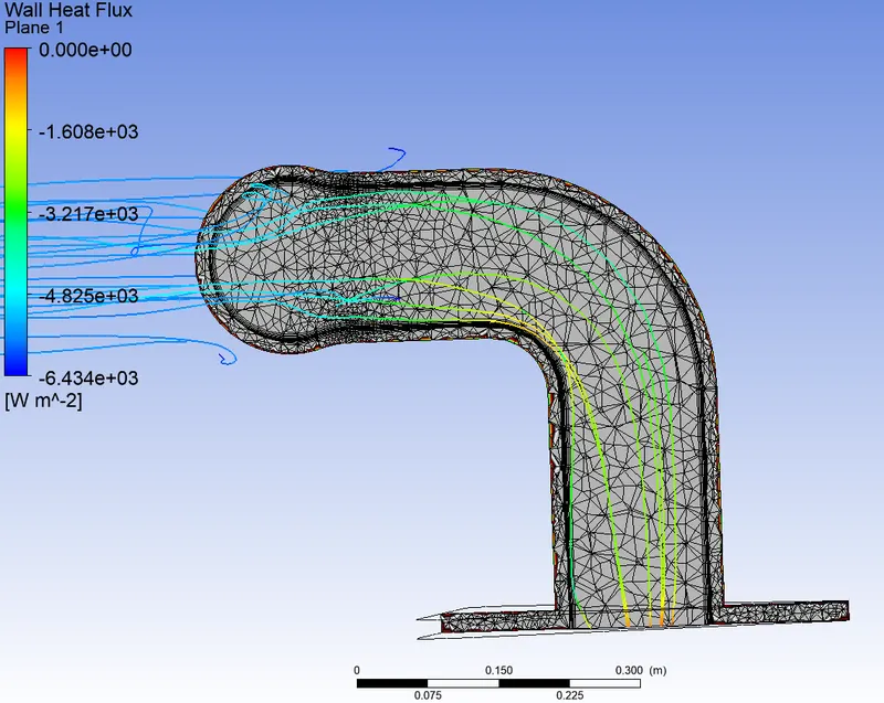
• And the velocity steamline 
  
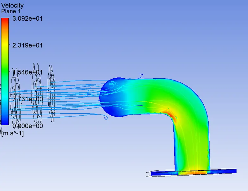
• Here, the maximum heat flux is observed at the location of turning point and also it is the maximum velocity is pointed. 

To verify if the HTC predictions from the simulations are right by using Analytical Calculation as shown below.

Reynolds number =ρ∗v∗Lμ">= (ρ∗v∗L )/μ       

= (1.225*5*0.17)/17894e-05

=58189.96

Here, the value of L is the characteristics length is taken as the inlet dia.

Here the value of Re is 58189.96 that means the flow is Turbulent. By using Dittus Bolter heat transfer coefficient relation we can determine the heat transfer coefficient value by determining the Nusselt number as follows;

NuD = 0.023∗Re^0.8∗Pr^n

where, Pr = (μ∗Cp)/k

μ = 1.7894e−05 kg/m.sec

k = 20 W/m^2.k

Cp = 1006.43 J/kg.k

so, Pr = (1.7894e−05*1006.43)/20 = 0.744

n is constant 0.3">0.30.3 heat transfer takes place from fluid to solid

Therefore, Nusselt number NuD = 136.48

Therefore convective heat transfer coefficient h = (Nu*k)/D = (136.48*20)/0.17 = 19.428 W/m^2.k

RESULTS AND COMPARISON:

• The Given model is stimulated by using, Ansys - Fluent under the Academic limits. Here, the stimulation is followed by the using pressure based steady solver used to discrete the geometry. 

Type of Mesh	No.of Elements	heat transfer coefficient  W/m^2.k
Baseline Mesh	171702	24.988108
refined mesh	404529	27.241283

The refined meshed module has the macimum velocity plots and the temperature distribution is also fine in this model

• And by using Analytical method we got the Heat transfer coefficient value as 19.428 W/m^2.k
• And the value of the heat transfer coefficient is located in the cell adjacent to the wall which allows us to choose the value of Y+ = 1
• And the velocity reaches maximum at the Turning point of the module and alos the Heat flux is also maximum at those locations. And the velocity at the outlet is higher than the velocity at the inlet, that can be  attributed to the presence of four inlets and one outlet.
• The accuracy of the model depends on the Analytical solution, Boundry conditions, material Properties, and also the geometry.
• From this CHT stimulation we predicated the Heat Transfer coefficient value of the given model and validated the value agaiinst the Analytical value with a deviation of range 5% - 10%, but these values are close to eachother.