Week 4 - CHT Analysis on Exhaust port
Aim: To perform conjugate heat transfer analysis over echaust port using ansys
Introduction about Conjugate heat transfer.
Conjugate heat transfer is a type of heat transfer analysis between solids and fluids. This type of heat transfer includes both convection(between fluids) and conductive(between solids) heat transfer as well as both forced and natural convection. CHT analysis can precisely predict heat transfer by simoultaneous solving all relevant solid and fluid flow heat transfer processes. The CHT approach therefore has benefits for those applications where heat transfer is either non uniform or difficulty to calculate.
Uses of CHT
The conjugate heat transfer methods have become a more powerful tool for modeling and investigating nature phenomena and enggineering systems in different areas ranging from aerospace and nuclear reactors to thermal goods treatment and food prcessing from comlex procedures in medicine to atomsphre thermal interaction in methodology.
Way to verify in the CHT prediction from the simulation.
Verify using available experimental data from the calclulation of nusselts number we can use calculate CHT
nu=0.023*(Re^(0.8))*Pr^n
Pr- prandti number
Re-Reynolds number
from the prandti number we can calculate the nusselts number
From the nusselts number we can calculate heat transfer coefficient
nu=(hD/k)
Accuracy
Accuracy depends on mesh size it majorly imoacts to simulation, finer mesh give accurate results. Refining of mesh contains more computational time. Inserting inflation layer are also gives aaccurate results and it helps perform bodyfitted mesh.
Steps involved in the simulation:
Geometry preparation:
Import Exhaust port geometry into spaceclaim
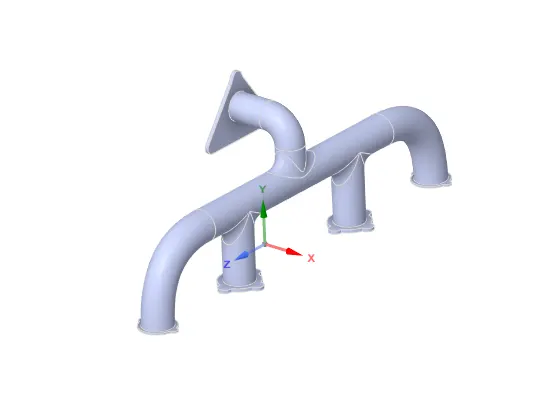
Volume Extrction
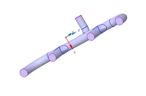
Extact fluid volume and solid volume using Volume extract toom and moved fluid volume and solid volume into new componets, delete empty components and enable share topology
Solid volume
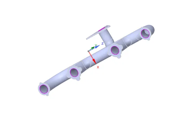
fluid volume
We need set share topology in set share and In workbench use share tool do share topollogy between solid volume and fluid volume, to know sharing we can see pink circle on the exhaust post
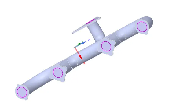
Meshing
Create name selection and mesh default element size
Element size:150 mm
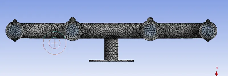
Simulation setup
Solver-steady time-Pressure based type-Absulute velocity
Viscous model-k epsilon (2eqn)
Material
- Fluid-Air
- Solid-Aluminium
Boudary condition-Inlet
- velocity 5m/s
- Thermal-700k
outer wall convection
- heat transfer coefficient-20 W(m2 K)
Solution
Define the plots what we need calulate like Heat transfer coefficient etc..
temperature contour
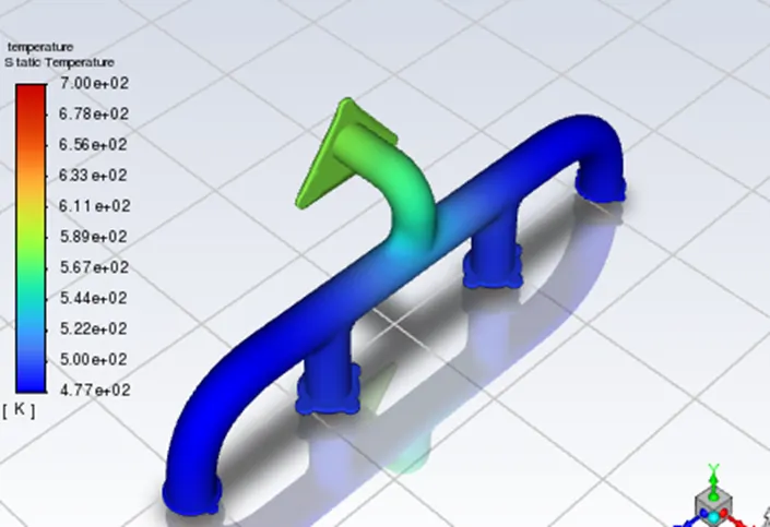
Velocity contour
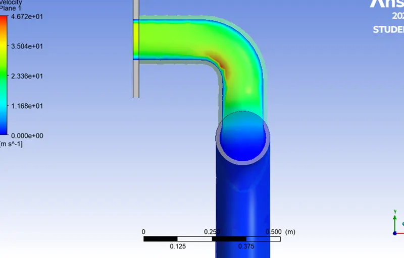
Velocity steamline
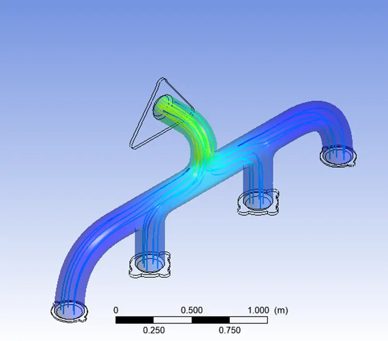
Heat transfer coefficient
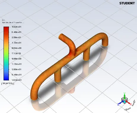
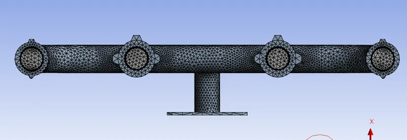
Refined mesh
Outer wall convection element size:70mm
Inner wall element size: 50mm
Inflation layer
- Total thickness:8mm
- growth rate:1.2
- Total layers: 8
Simulation setup
Solver-steady time-Pressure based type-Absulute velocity
Viscous model-k epsilon (2eqn)
Material
- Fluid-Air
- Solid-Aluminium
Boudary condition-Inlet
- velocity 5m/s
- Thermal-700k
outer wall convection
- heat transfer coefficient-20 W(m2 K)
Solution
Define the plots what we need calulate like Heat transfer coefficient etc..
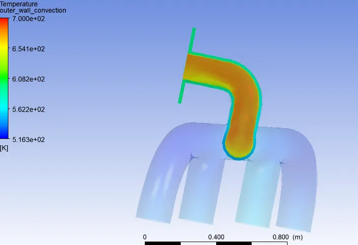
Temperature contour
Velocity contour
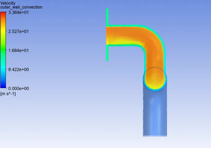
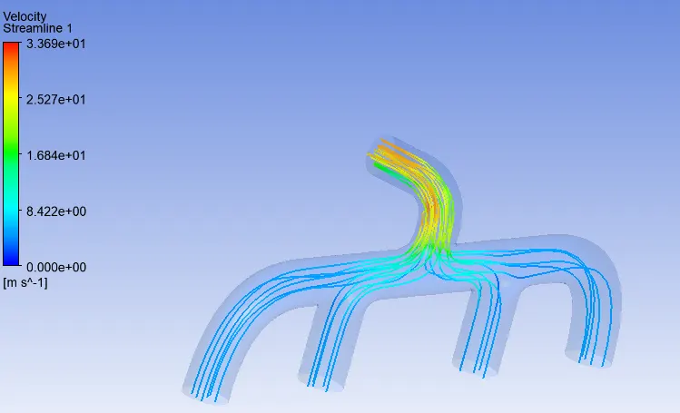
Velocity steamline
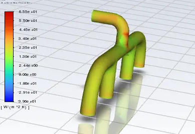
Heat transfer coefficient
Results
Average Heat transfer coefficient
| Mesh type | Heat transfer coefficient W(m2 K) |
| Default mesh | 21.22 |
| Refined Mesh | 20.66 |
Conclution
- Default element size mesh take less time and refined mesh takes longer time
- When we refining mesh the heat transfer coeffiecient is decreases
- Finally CHT anlysis on Exhaust port simulation perfoemed succesfully and results are ploted.