Week 4 - CHT Analysis on Exhaust port

AIM

To do the conjugate heat transfer simulation of an exhaust port and calculate the heat transfer coefficient. Show velocity and temperature contours and validate the result.

CHT Analysis

The conjugate heat transfer analysis helps to do the simulation of heat transfer between solid and fluid domains by exchanging exchanging thermal energy at the interfaces between them. Applications of this analysis type helps in the design of heat exchangers, cooling of electronic equipment, and general-purpose cooling and heating systems. CHT Simulations help in effieciently designing systems where conductive and convective heat transfer occur and helps reduce the cost and time of development by obtaining an optimized design for testing.

Y+ Value

y+ is a non-dimensional distance. It is often used to describe how coarse or fine a mesh is for a particular flow pattern. It is important in turbulence modeling to determine the proper size of the cells near domain walls. The turbulence model wall laws have restrictions on the y+ value at the wall.

For inlet velocity of 5 m/s and inlet diameter of 166.1 mm, the reynolds number is 56900. Using K-epsilon model for heat transfer, we can select the y+ criteria as 1<y+<5

For a y+ value of 5, we can calculate the first layer of mesh thickness from using the y+ calculator.

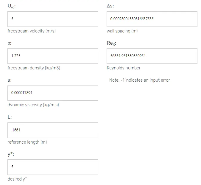
The first layer thickness can be 2 mm from the calculation. So we can use total thickness of 5 mm with 5 layers of inflation and a scale factor of 1.2 for the simulation.

Procedure

• Import the geometry into spaceclaim.
• Use Prepare>volume extract tool and select the edges if inlets and outlets to extract the volume.
• Once the fluid volume is extracted, move solid and fluid volume under a single component.
• Use share option in Workbench>share to have information transfer between fluid and solid volumes and we get confromal mesh during the meshing process.

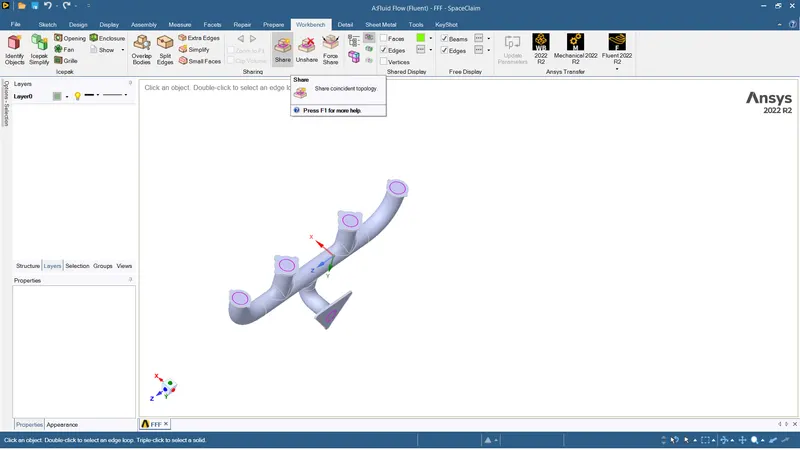
• Close the spaceclaim and update mesh in the fluid workbench.
• Open mesh module.
• Create named selections for the geometry.
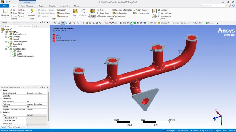
• First we will do a baseline simulation with default mesh of ansys.
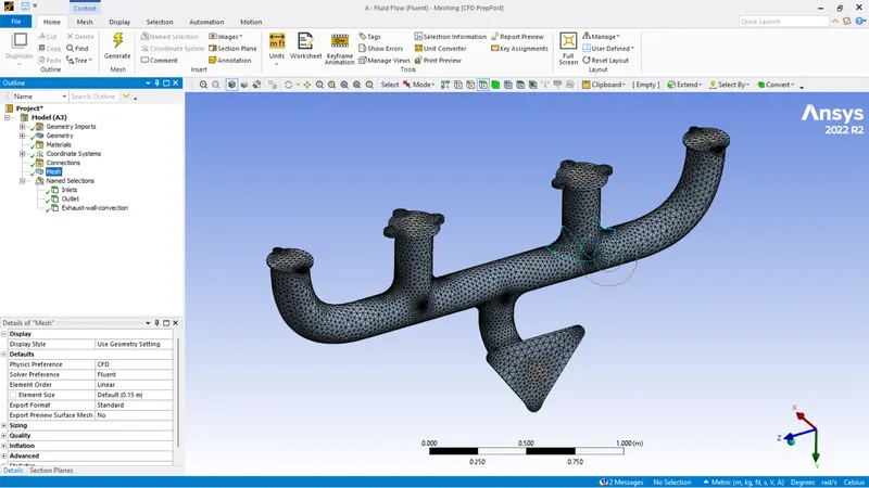
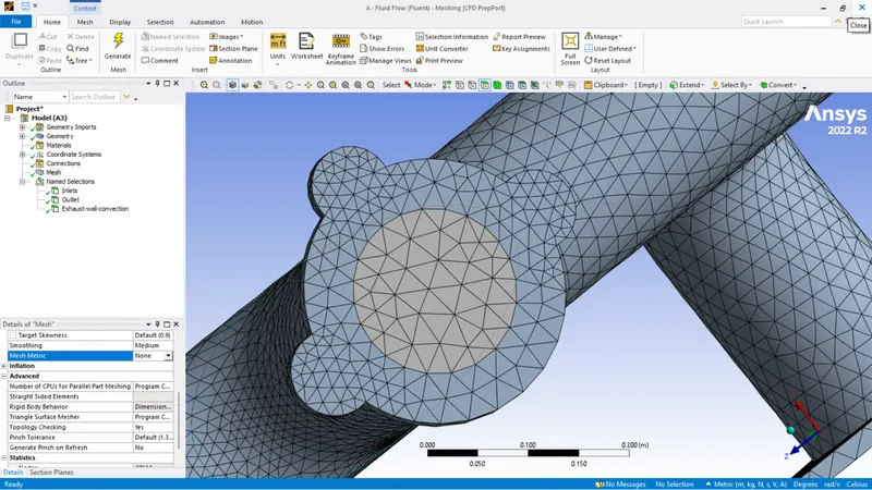
• Element size : 150 mm; Nodes : 27512; Elements : 138053
• The mesh is conforming and there is no gap at the solid and fluid interface.
• Close the mesh module.
• Open setup with double precision.

Solver	Pressure Based
Velocity Formulation	Absolute
Time	Steady
Energy	On
Viscous model	Standard K-Epsilon with standard wall function
Materials	Solid : Aluminium; Fluid : Air
Cell Zones	Exhaust Solid type : Solid; Exhaust volume : Fluid
Solution method	Coupled

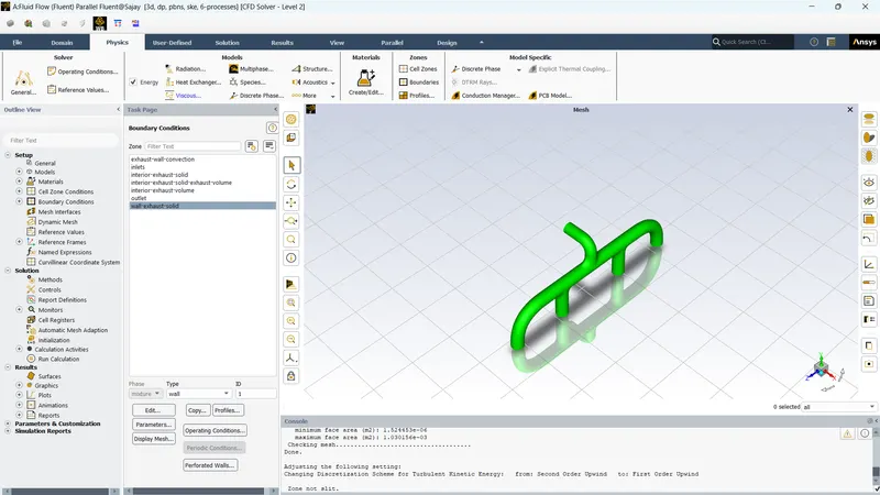
Boundary conditions were updated as :

Inlets	Velocit inlet; Velocity magnitude : 5 m/s; Thermal : 700 K
Outlet	Pressure Outlet; Gauge pressure : 0 Pa; Thermal : 300 K
Outer wall convection	Convection; Heat transfer coefficient : 20 W/m2K; Free steam temp : 300 K
Wall exhaust solid	Heat Flux : 0 W/m2
Interiors	interior

The solution was initialized using hybrid initialization and run for 300 iterations.

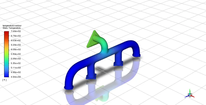
Streamlines coloured with velocity starting from inlet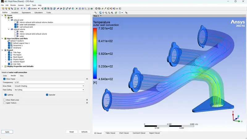

surface heat transfer coefficeint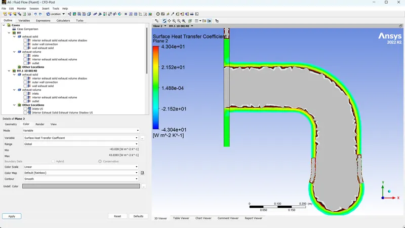

The heat transfer coefficient was about 43 W/m2K.

The same setup was run with a refined mesh and inflation layer.

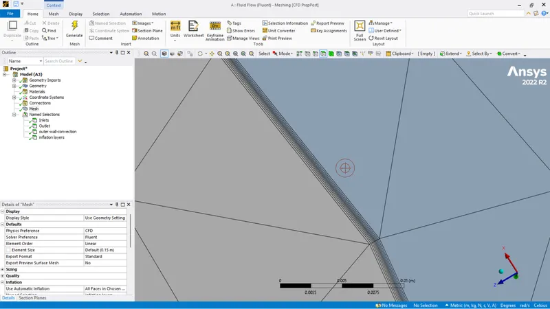
Body sizing was given to the exhaust port

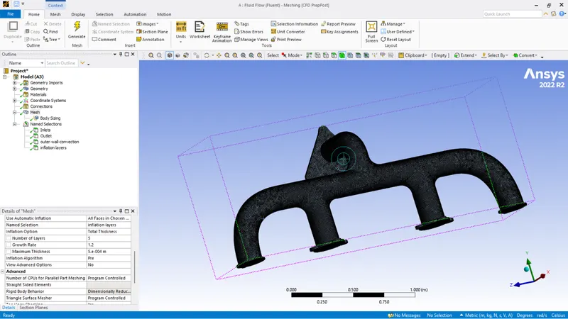
Nodes : 131644; Elements : 414739

Simulation was run for 300 iterations with same setup.

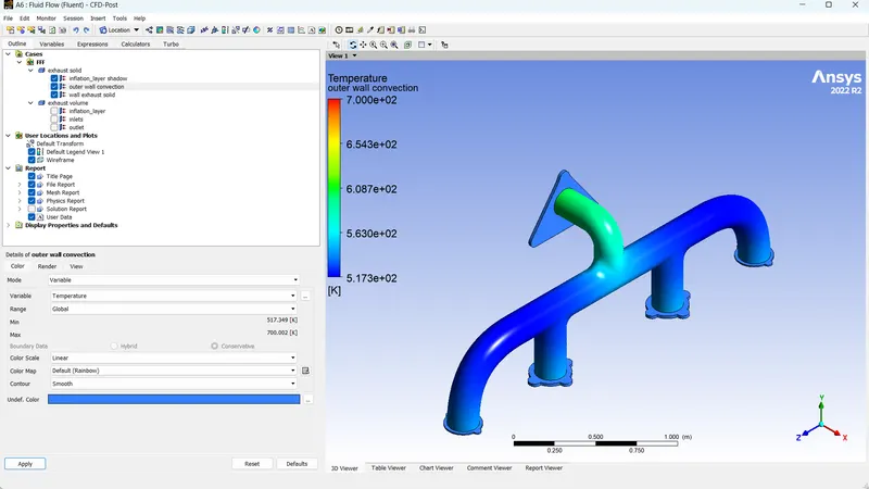
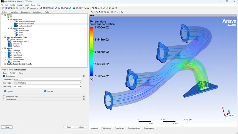
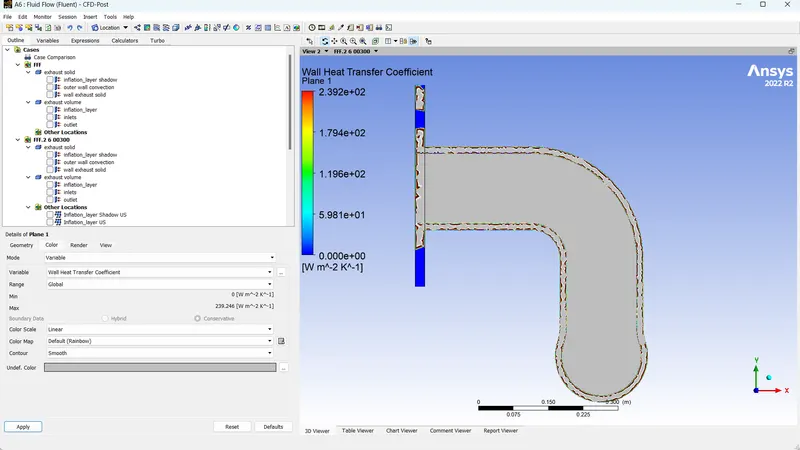
The wall heat transfer coeffcient had a value of 239.2 W/m2K.

Forced convection of gases have heat transfer coefficient of 200-300 W/m2K

Conclusion

The highest velocity is observed at the bend of the outlet. Also the heat transfer coefficient plot shows the highest value at the highest velocity region.

Refining the mesh improved the definition of the results but also increased the computational time drastically.