Week 4 - CHT Analysis on Exhaust port

Aim: To Simulate Conjugate Heat Transfer (CHT) Analysis On Exhaust Port.

Objective:

• Theory Explanation
• Mesh Refinement Up To Maximum Limit
• Figure It Out Streamline And Boundary Wall Heat Transfer

Theory:

The Conjugate Heat Transfer (CHT) Analysis Type Allows for The Simulation of Heat Transfer Between Solid And Fluid Domains By Exchanging Thermal Energy At The Interfaces Between Them. The Simulation Of The Heat Exchangers, Cooling Of The Electronic Equipment, And General-Purpose Cooling And Heating System. In Solids, Conduction often Dominates whereas, In Fluids, Convection Usually Dominates. This Type Of Heat Transfer Includes Both Convection And Conductive Heat Transfer, As Well As Both Forced And Natural Convection. Which Is More Stable And Provides Faster Convergence As The Energy Equation Is Strongly Coupled Between The Solid And Fluid Regions.

Geometry:

1. Import the model into new space claim then change the units into meters.
2. Select the repair tool and use the extra edges command to remove the unwanted edges.
3. Select the prepare tool and use the volume extract command to extract the model.
4. Name them as fluid and solid volumes and make them as a single model component ,then enable the share topology to achieve the confirmed detail mesh between the fluid and solid volumes.
5. Finally ,Select the workbench tool and use the share command to share the properties of the fluid to achieve conjugate heat transfer (CHT) .

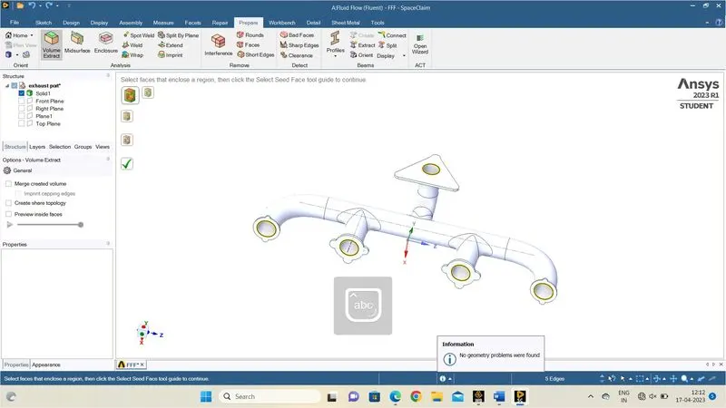
Before volume extraction

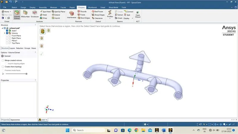
After volume extraction

Mesh:

Meshing is the process of discretization of the simulation domain. That means we split up a large domain into multiple smaller domains and solve equations for them .a multi region mesh is required for a CHT simulation to have a clear definition of the interfaces in the computational domain.

• After update the geometry give name selection according to model.
• After name selection ,generate the base mesh to the model.
• After the base mesh generation ,use the inflation for the fluid model.
• After the inflation ,insert body size mesh to get better mesh refinement up to maximum limit.

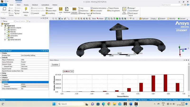
Base mesh

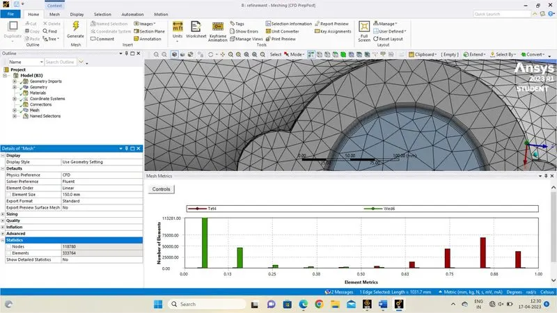
Refine mesh

Fluent setup:

• After Updating The Mesh Open Fluent Setup, Select A Pressure-Based Solver Using The Steady-State Time Simulation And Absolute Velocity Formulation Under The General Settings.
• Under The Physic Choose The Energy Option As We Are Dealing With Temperature Properties.
• Input The Boundary Values, 5 M/S As Inlet Velocity At 700K. Set The Outer Wall Convection Boundary To Convection Type And Input Constant Value Of Heat Transfer Coefficient As 20.
• Under Materials, Choose Air As The Fluid material And Aluminium As Solid Material.
• Enter The Reference Value As Per The Geometry And Inlet Boundary Conditions.
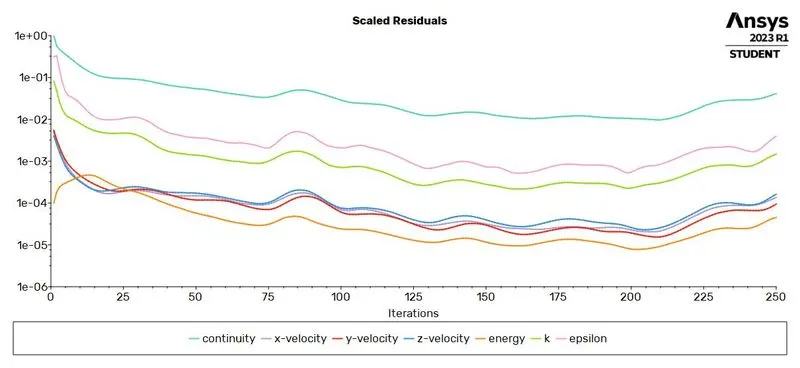
• Initialize The Hybrid Initialization And The Simulation For 250 Iterations.

CASE 1: BASE MESH SIMULATION

• Element Size: 100mm
• Of Element: 138398
• Viscous Model: K-Epsilon
• Inlet Velocity: 5m/S
• Inlet Temperature: 700k
• Heat Transfer Coefficient: 20 W/m^2K

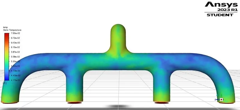
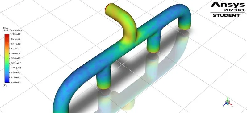
TEMPERATURE DISTRIBUTION:

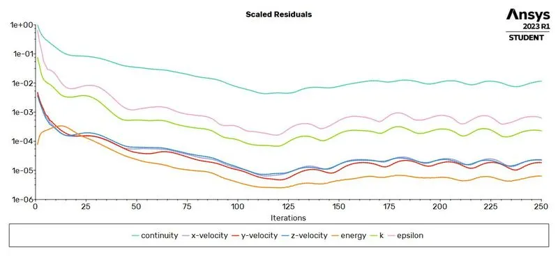
RESIDUAL PLOT:

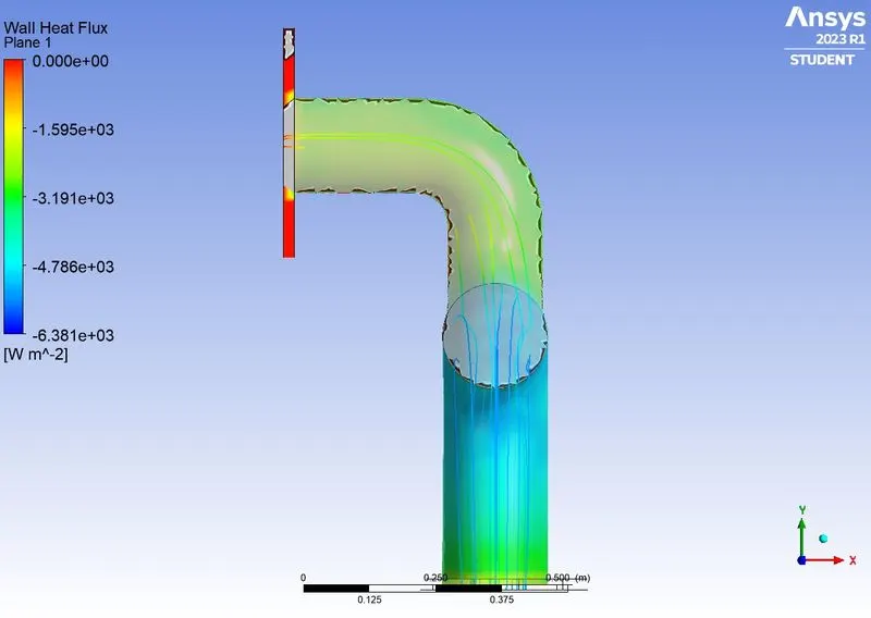
WALL HEAT TRANSFER COEFFICIENT:

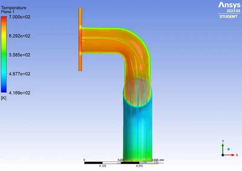
TEMPERATURE COUNTOUR:

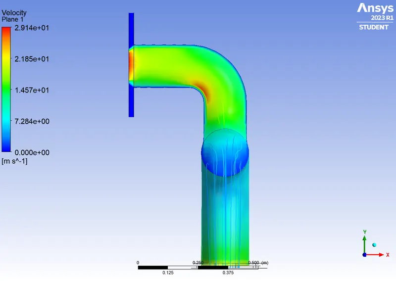
VELOCITY COUNTOUR:

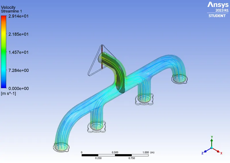
VELOCITY STREAMLINE PLOT:

CASE 2: REFINE MESH SIMULATION

• Element size: 150mm
• Sizing Element size: 20mm
• of Element: 332433
• Viscous Model: K-epsilon
• Inlet Velocity: 5m/s
• Inlet Temperature: 700K
• Heat transfer coefficient: 20W/m^2k

TEMPERATURE DISTRIBUTION:

RESIDUAL PLOT:

WALL HEAT TRANSFER COEFFICIENT:

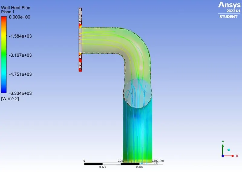
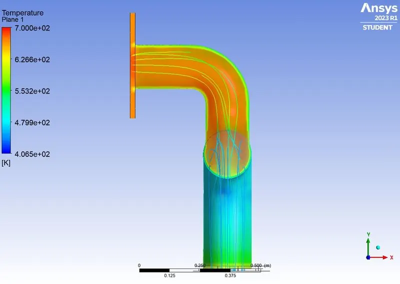
TEMPERATURE COUNTOUR:

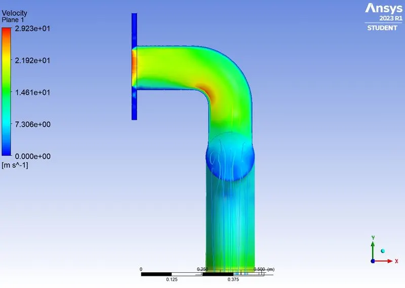
VELOCITY COUNTOUR:

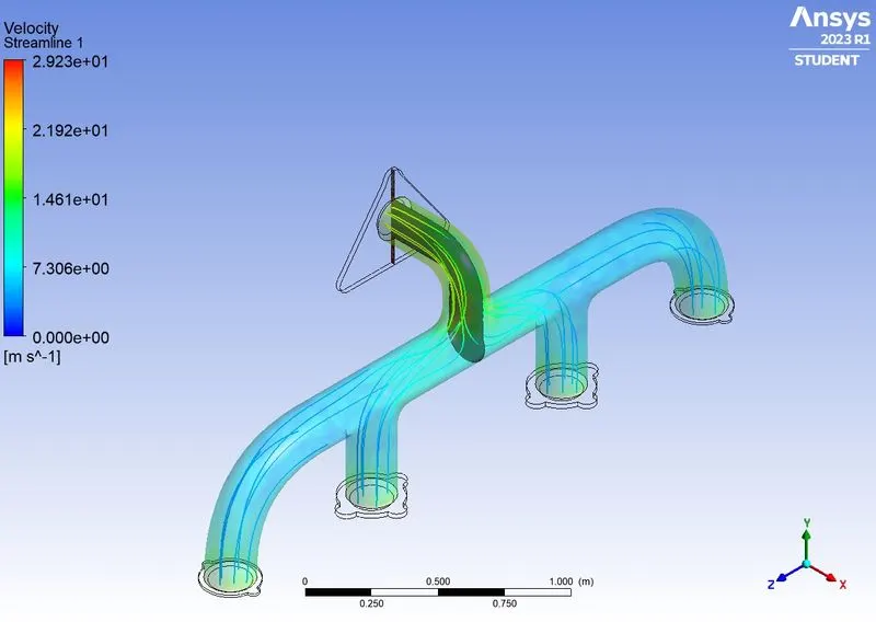
VELOCITY STREAMLINE PLOT:

CASE 3: REFINE MESH SIMULATION

• Element size: 150mm
• Sizing Element size: 20mm
• of Element: 332433
• Viscous Model: K-omega
• Inlet Velocity: 5m/s
• Inlet Temperature: 700K
• Heat transfer coefficient: 20W/m^2k

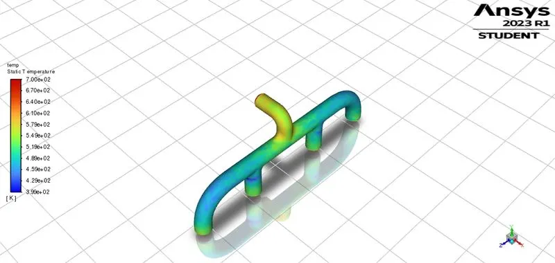
TEMPERATURE DISTRIBUTION:

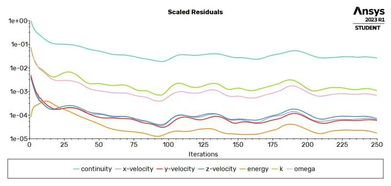
RESIDUAL PLOT:

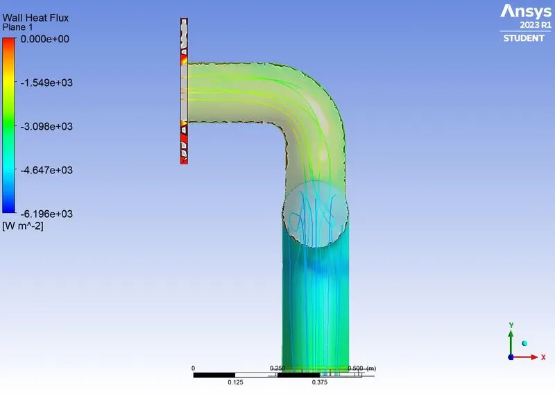
WALL HEAT TRANSFER COEFFICIENT:

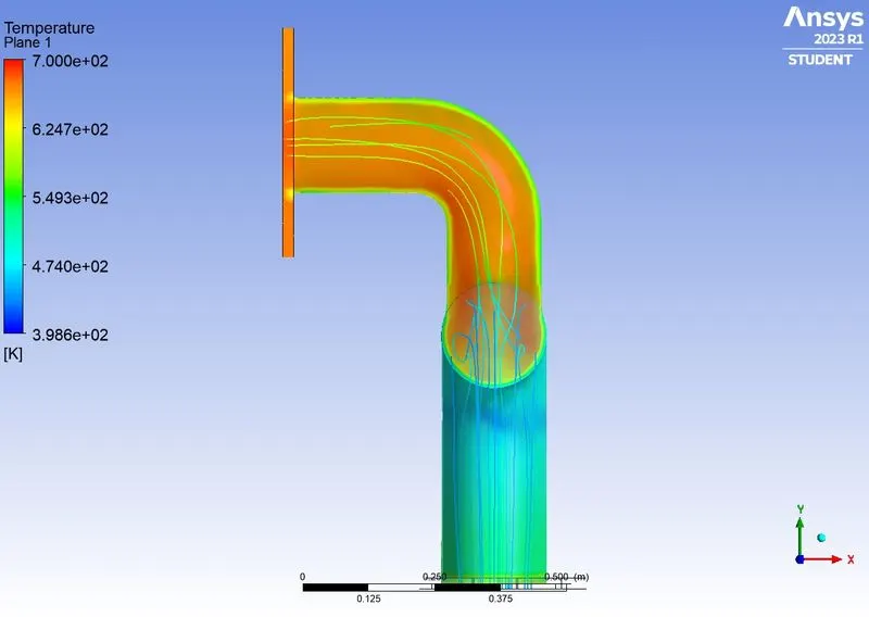
TEMPERATURE COUNTOUR:

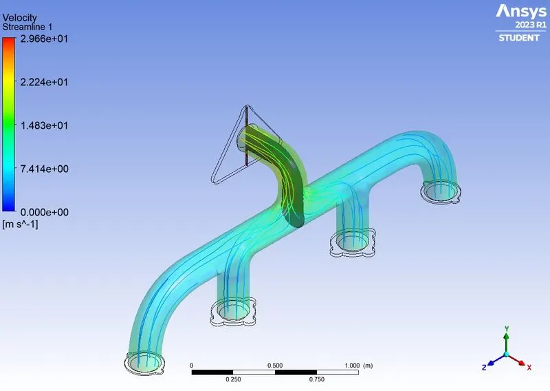
VELOCITY COUNTOUR:

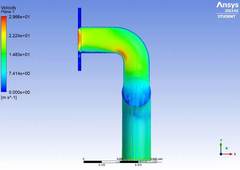
VELOCITY STREAMLINE PLOT:

How would you verify if the htc predictions from the simulations are right? On what factors does the accuracy of the prediction depend on?

According to bernoulli's mass conservation principle mass is conserved in our model which is clearly explained below;

Let us assume the flow rate from each inlet as q1, q2, q3, q4 respectively, and q5 be the flow rate from the exhaust manifold.

As mass is neither created nor destroyed, mass flow rates are also balanced as below;

Q1+q2+q3+q4=q5 ...........(1)

We have q= ρ⋅a⋅v ...........(2)

Now equation 1 becomes

A1v1+a2v2+a3v3+a4v4=a5*v5

As it is an incompressible flow to compensate for mass flow, velocity is increased. And the overall mass flow rate is conserved.

As velocities are high, the reynolds number at the outlet manifold will be high.

Nu=f(re,pr) for forced convection application.

Nu= hdkℎ

From above formula nudirectly∝ re. Hence nu∝∝h, therefore, re∝∝h.

From our simulation, we have observed velocities are high at bend section of outlet manifold hence higher reynolds number which was at high heat transfer coefficient. Therefore predictions from our simulations can be considered correct.

Factors that influence accuracy of predictions:

Mesh Quality Greatly Impacts The Accuracy Of Prediction Value In Our Simulations Which Can Be Observed From Above Contours And Maximum Values Of Related Parameters Like Velocity And Heat Transfer Coefficient.

An Appropriate Turbulence Model Has To Be Used In Accordance With The Y+ Value Which Is Very Important.

Appropriate Y+ Value Helps In Calculating Total Layer Thickness From The Wall For The Better Capturing Of Effects Near Wall, Which Is Heat Transfer Coefficient In Our Case.