Week 4 - CHT Analysis on Exhaust port

CONJUGATE HEAT TRANSFER ANALYSIS ON EXHAUST PORT

AIM:

To perform Conjugate Heat Transfer (CHT) analysis on an exhaust port and evaluate the average surface heat transfer coefficient and compare the results with the analytical solution.

THEORY:

Conjugate Heat Transfer analysis:

The Conjugate Heat Transfer (CHT) analysis allows us to study the heat transfer occurring between solid and fluid. It involves the variations of temperature within solids and fluids, due to thermal interaction between the solids and fluids.

As evident, conduction often dominates in solids and convection usually dominates in case of fluids. Efficiently combining the heat transfer in fluids and solids helps in effective designing of heaters, coolers, or heat exchangers. The applications of these type of simulation can be extended further to study heat transfer occurring in heat exchangers, cooling of electronic equipment, general-purpose cooling and heating systems and much more.

One such application is the study of CFD analysis performed to evaluate the temperature and velocity distribution for an inline 4-cylinder exhaust port. The study focuses to determine the temperature distribution and the wall heat transfer coefficient at the exhaust port.

PROCEDURE:

Geometry:

• Create a fluid flow (fluent) project in Ansys Workbench.
• Import the ‘exhaust port’ geometry to ‘Space Claim’ interface.

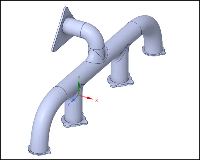
• Extraction of fluid volume using ‘edge selection’.

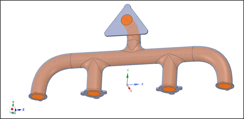
• Now close space claim and open ANSYS Mesher and click on generate mesh.

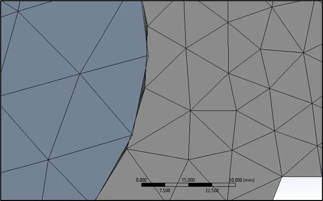
• The overall mesh seems to be correct but if zoomed in for inlets and outlet, a non-conformal mesh can be observed meaning the mesh vertices of both the volumes are not intersecting and this needs to be fixed in order to obtain a smoother transfer of heat.
• Clear the mesh generated and open space claim.
• Right click on ‘exhaust port’ and click on ‘create new component’ to include both solid and fluid volume. Delete the existing empty components.

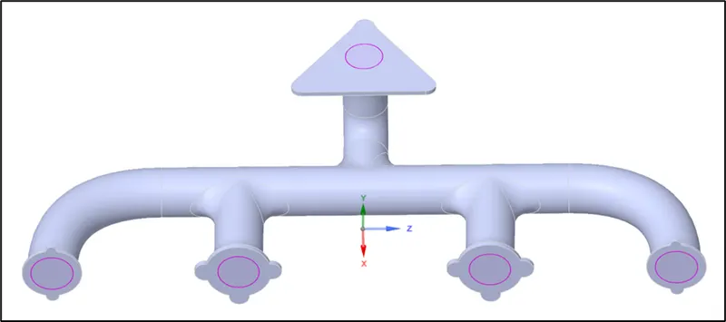
• Click on workbench menu and click on ‘share’ option. This step ensures that the interfaces of the selected volumes are seen when shared and the mesh obtained will be a conformal mesh meaning the vertices of both the volumes will intersect.
• The highlighted purple colour shows that the interfaces are shared.

Mesh:

Case 1: Baseline mesh

• Create named selection

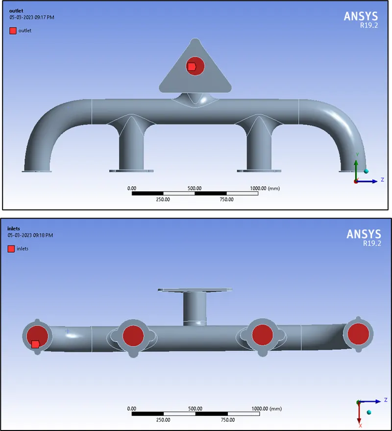
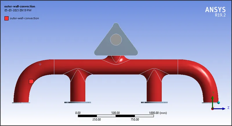
• All the remaining walls are default set by fluent as adiabatic boundaries.
• Click on generate mesh.
• The mesh is generated for an element size of 150 mm (default). The number of elements is 138485 of tetrahedral type with an average element quality of 0.819.

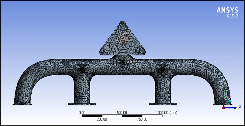
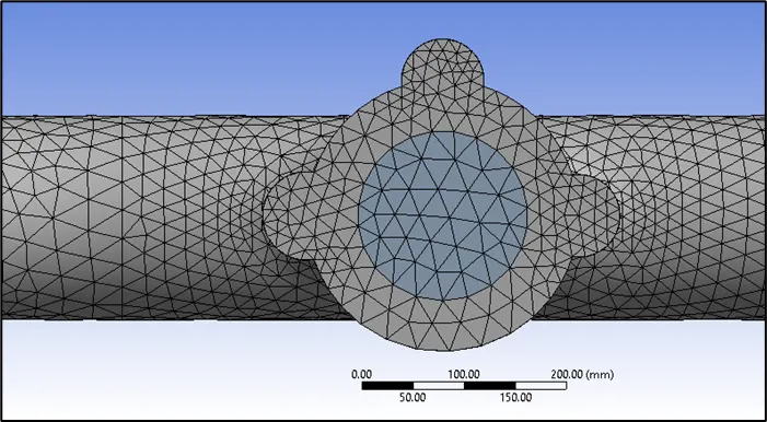
• It is also observed that the mesh is conformal at the solid fluid interface meaning the elements of both volumes are connected to each other, which will result in a smooth heat transfer.

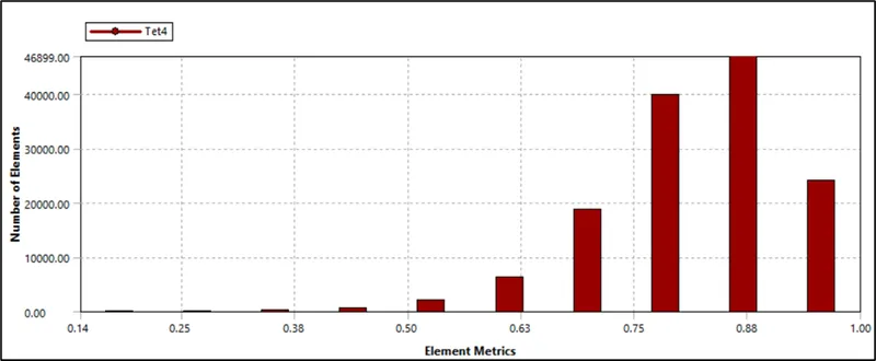
• The mesh metrics is also above 0.10 which is acceptable for this simulation.

Simulation setup:

• Steady state pressure-based solver with absolute velocity formation.
• The simulation is carried out by enabling energy equation and using ‘k-omega SST’ turbulence model, since it is best suited for simulations near the wall and includes the effect of the 'k-epsilon' model also.

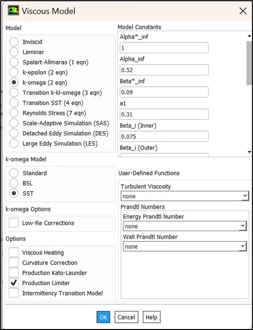
• The fluid material is set as ‘air’ and the solid material is set as ‘aluminium.’

Boundary conditions:

Inlet:

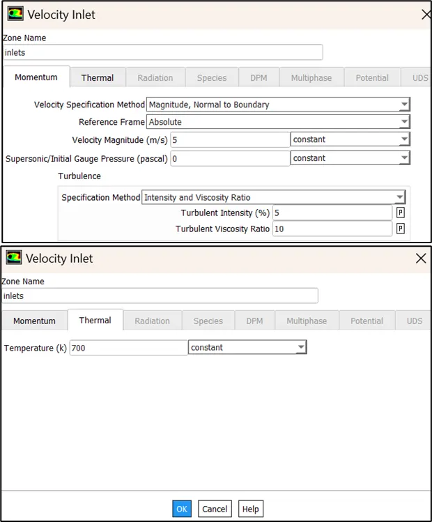
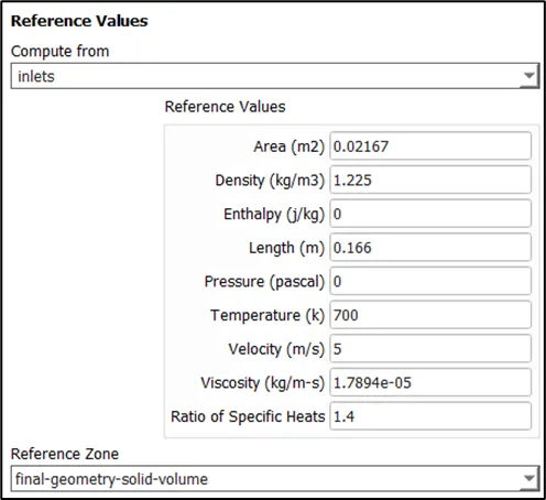
• Velocity = 5 m/s; temperature = 700 K

Outer wall convection:

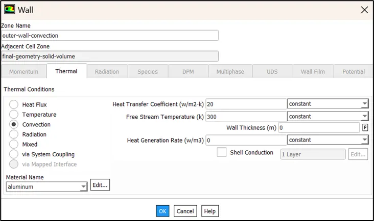
• Heat transfer coefficient = 20 W/m-K.

Outlet: Default boundary conditions

Reference values

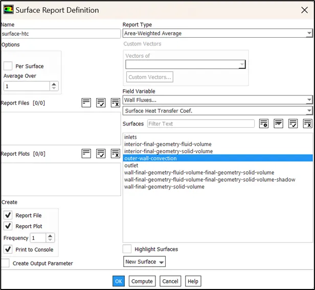
• Report definition for average surface heat transfer coefficient.

• Initialize the solution using ‘hybrid initialization’ method.
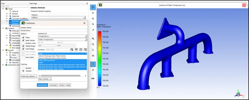
• Create ‘temperature contour’ to monitor the temperature at the outlet.

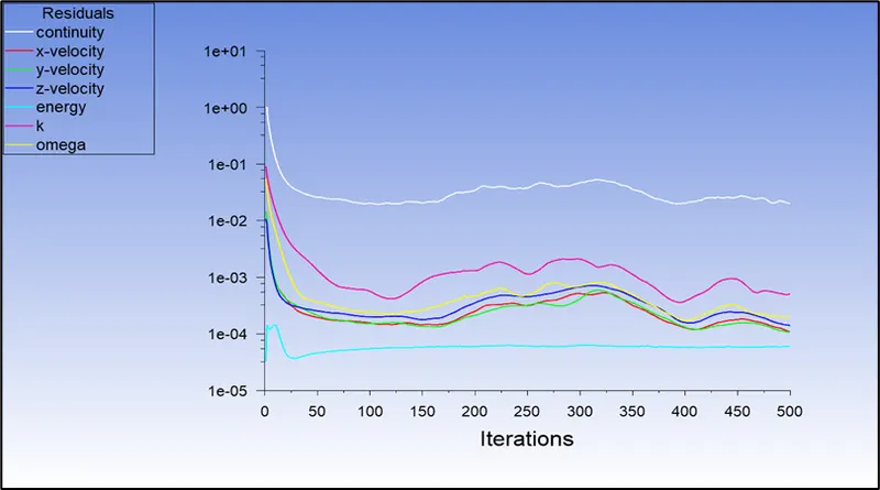
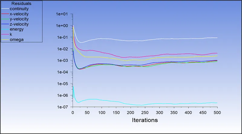
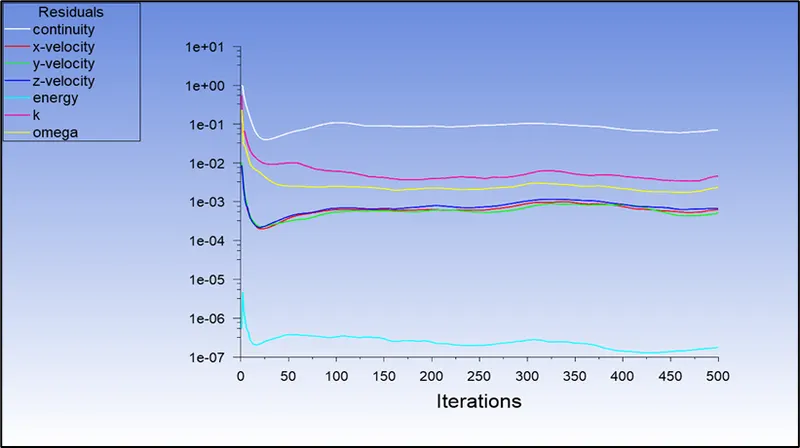
• Initialize the solution using hybrid initialization and run the simulation for 500 iterations.

Residual plot

Temperture contour plot

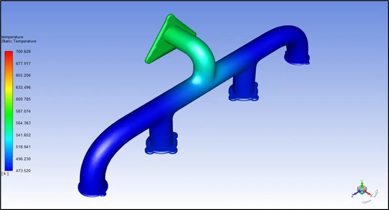
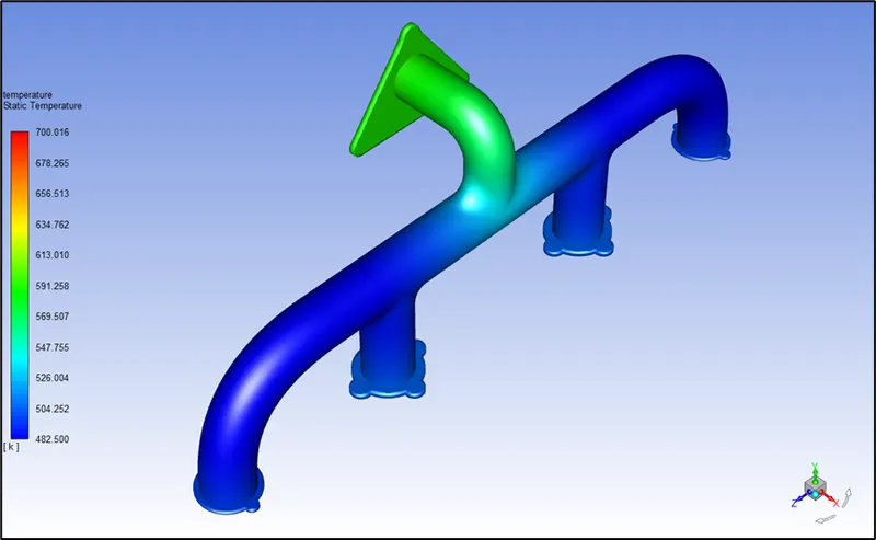
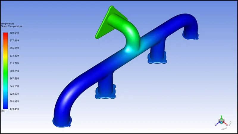
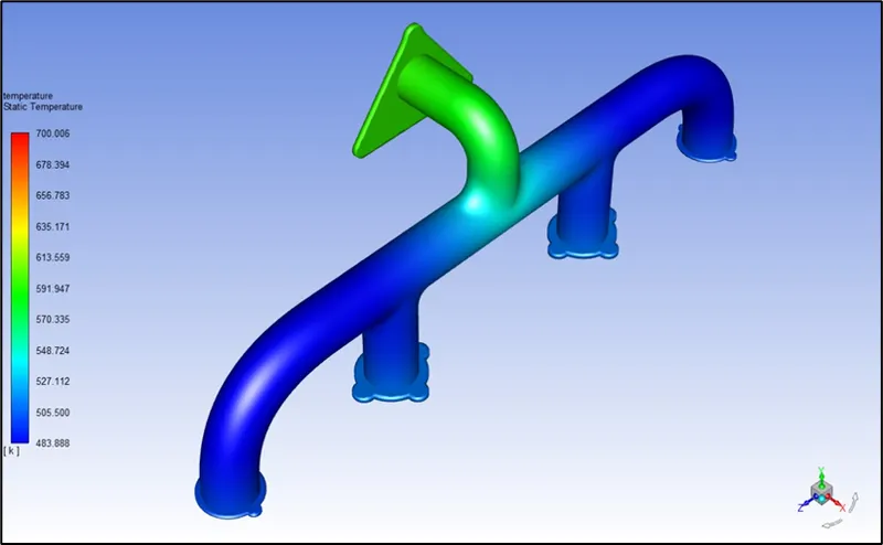
• As observed from the temperature contour, ideally the temperatures near the inlets are expected to be higher than outlet, but here due to convection the temperature at the outlet is higher than the inlets. To understand this better, consider the velocity plot.

Velocity contour plot

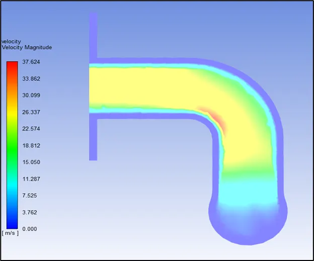
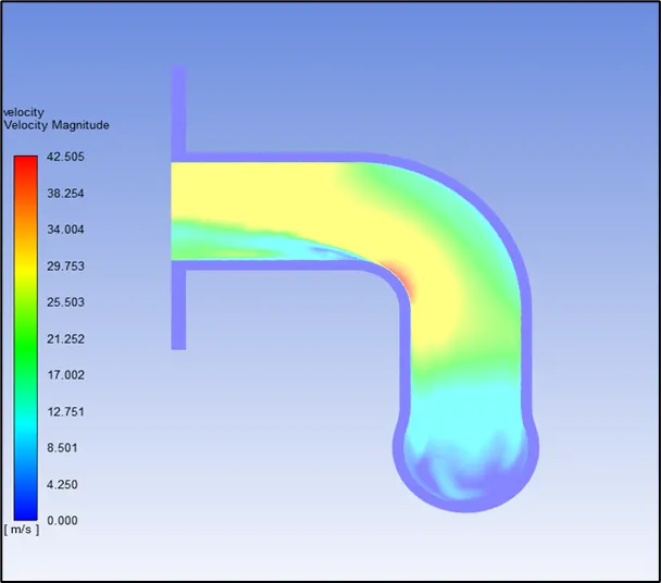
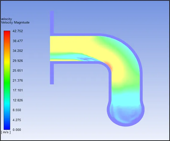
• It is observed that the velocity at the outlet is higher at the outlet, this happens because of the law of conservation of mass (Q = A.V). Since, there are 4 inlets and only 1 outlet and the total amount of air that has entered must flow out, the velocity at the exit is higher. This also can be inferred as a higher value of Reynolds number in that region, higher heat transfer coefficient, higher heat transferred from the fluid to the solid and hence higher temperature.

Average surface heat transfer coefficient

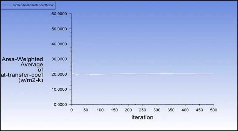
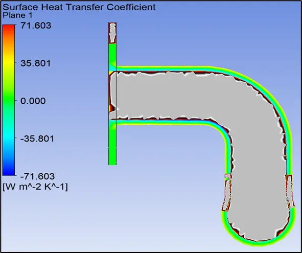
The average surface heat transfer coefficient is 20.023 W/m²-K and the maximum surface heat transfer coefficient is 75.376 W/m²-K.

MESH REFINEMENT

The further study is carried out by refining the mesh by inserting face sizing of 10 mm. The simulations are carried out for 500 iterations using viscous model k-omega SST (effective in predicting near wall results). The Y+ values are considered to be between 1 and 5, so that the solver uses equations of viscous sublayers and to obtain more accurate results Y+ can be less than or equal to 1 (source: Ansys fluent theory guide).

CASE 1

Y+ = 1;

Growth rate = 1.2;

Inflation layers = 25;

Element size = 10 mm

First layer thickness calculation

Inlet diameter of pipe = 0.166 m

Density of air = 1.225 Kg/m³

Velocity of fluid = 5 m/s

Dynamic viscosity = 1.7894*10^-5 Kg/m-s

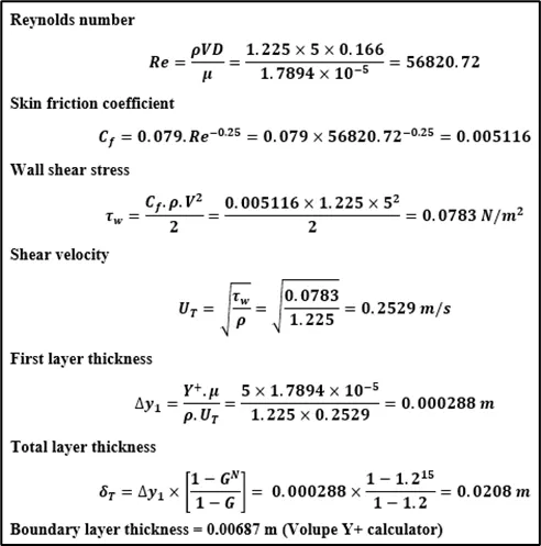
Reynolds number

Skin friction coefficient

Wall shear stress

Shear velocity

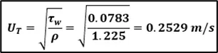
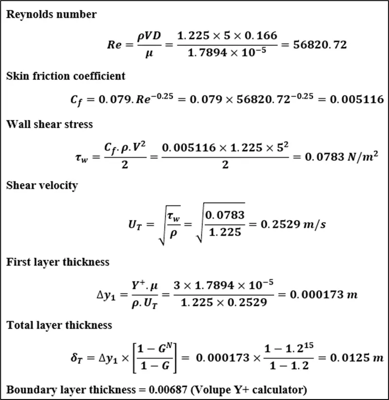
First layer thickness

Total layer thickness

Boundary layer thickness = 0.00687 m (Volupe Y+ calculator)

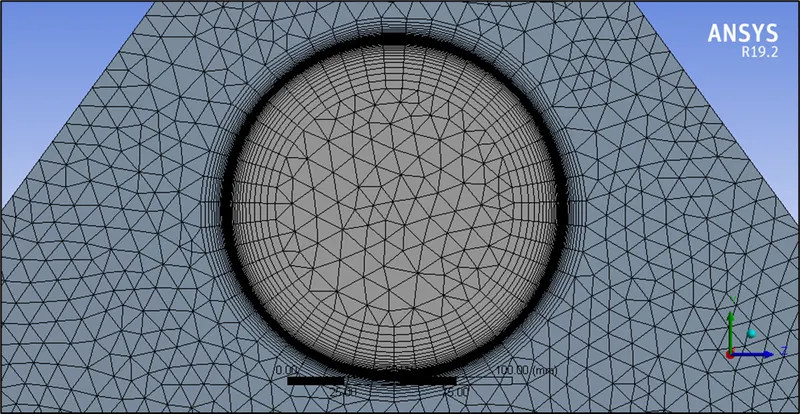
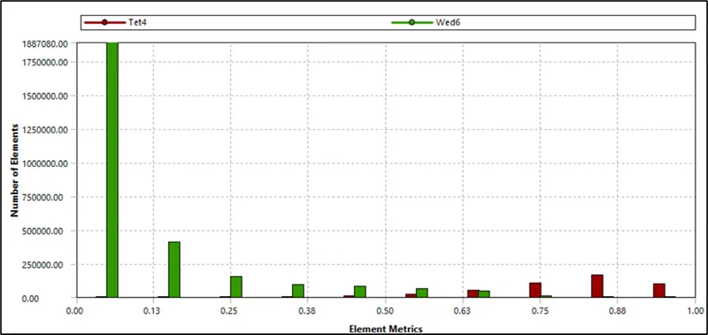
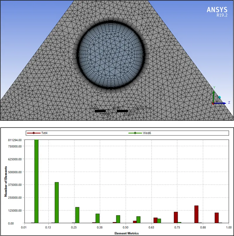
Mesh and mesh metrics

No. of elements = 3081849; average element quality = 0.309

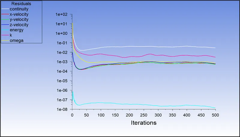
Residual plot

Temperature contour plot

Velocity contour plot

Average surface heat transfer coefficient

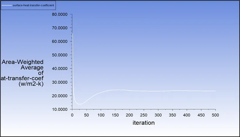
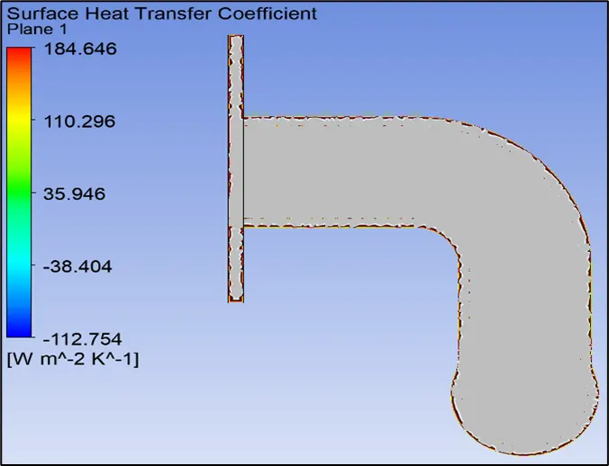
The average surface heat transfer coefficient is 23.381 W/m²-K and the maximum surface heat transfer coefficient is 184.646 W/m²-K.

CASE 2

Y+ = 3; Growth rate = 1.2; inflation layers = 15; element size = 10 mm

First layer thickness calculation

Inlet diameter of pipe = 0.166 m

Density of air = 1.225 Kg/m³

Velocity of fluid = 5 m/s

Dynamic viscosity = 1.7894*10^-5 Kg/m-s

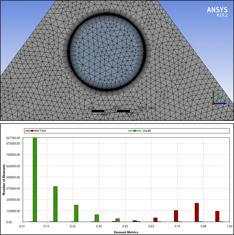
Mesh and mesh metrics

No. of elements = 2789316; average element quality = 0.314

Residual plot

Temperature contour plot

Velocity contour plot

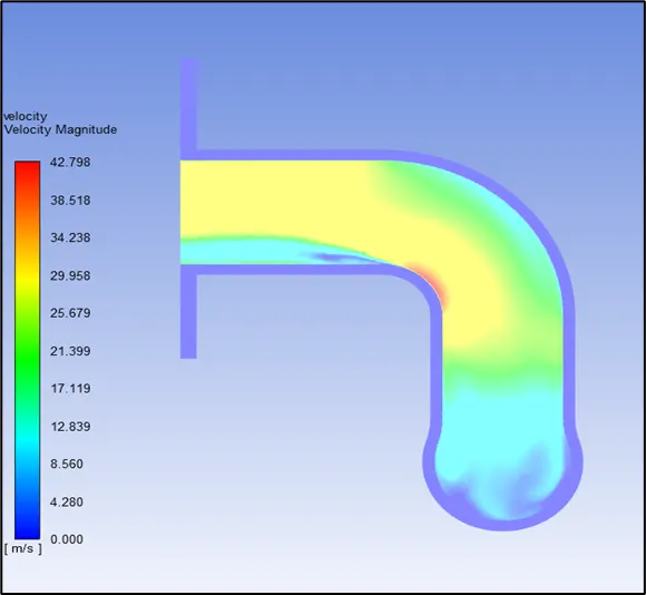
Average surface heat transfer coefficient

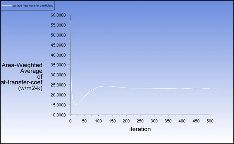
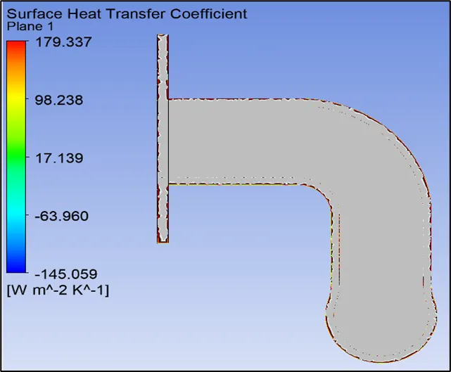
The average surface heat transfer coefficient is 23.901 W/m²-K and the maximum surface heat transfer coefficient is 179.337 W/m²-K.

Case 3

Y+ = 5; Growth rate = 1.2; inflation layers = 15; element size = 10 mm

First layer thickness calculation

Inlet diameter of pipe = 0.166 m

Density of air = 1.225 Kg/m³

Velocity of fluid = 5 m/s

Dynamic viscosity = 1.7894*10^-5 Kg/m-s

Mesh and mesh metrics

No. of elements = 2636856; average element quality = 0.316

Residual plot

Temperature contour plot

Velocity contour plot

Average surface heat transfer coefficeint

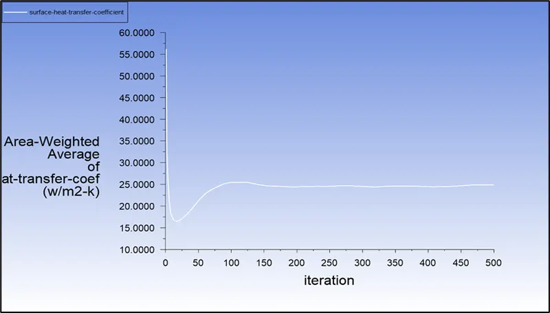
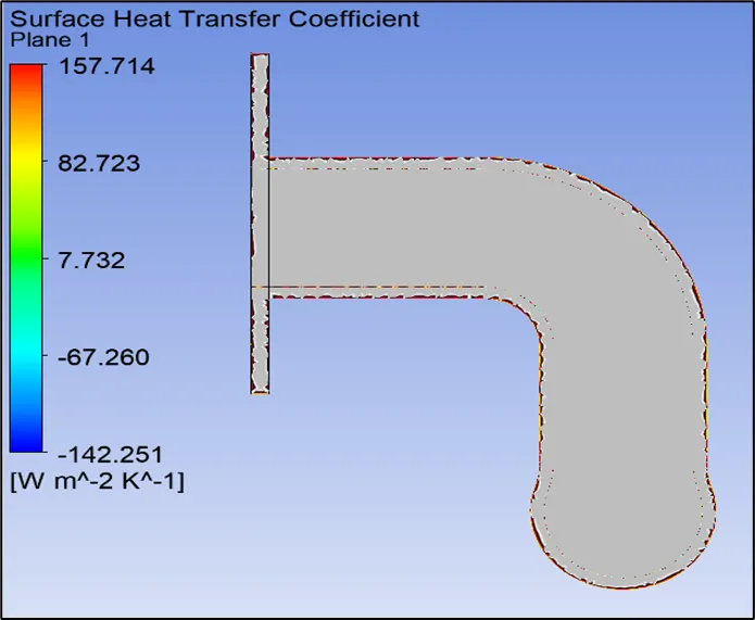
The average surface heat transfer coefficient is 24.889 W/m²-K and the maximum surface heat transfer coefficient is 157.714 W/m²-K.

VALIDATION FOR SURFACE HEAT TRANSFER COEFFICIENT

Using Dittus – Boelter equation

where,

• Reynolds number, Re = 56820.72
• n = 0.3 (for cooling of fluid)

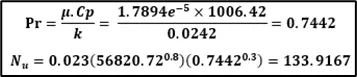
Average surface heat transfer coefficient,

Sl. No	Element size (mm)	Y+ value	No. of inflation layers	No. of elements	Average element quality	Velocity (m/s)	Average surface heat transfer coefficient (W/m2-K)	% error
1	150 (default)	-	-	138485	0.819	37.624	20.023	2.497
2	10	1	25	3081849	0.309	42.505	23.381	16.50
3	10	3	15	2789316	0.314	42.798	23.901	18.317
4	10	5	15	2636856	0.316	42.752	24.889	21.559

RESULTS AND CONCLUSION

The conjugate heat transfer (CHT) analysis for an exhaust port is performed to evaluate the average surface heat transfer coefficient. The evaluated vales through simulations are validated using Dittus-Boelter equation. The conclusions are as follows:

• The temperatures at the outlet is higher than the inlet because of the conservation of mass. Further, the velocity is found to be maximum at the bent section of the outlet. Hence, we obtain a maximum Reynolds number at that region, maximum heat transfer coefficient and maximum heat transfer at that region.
• The average surface heat transfer coefficient calculated from Dittus Boelter equation is well in agreement with the assumed heat transfer coefficient value.
• The average surface heat transfer coefficient obtained through different Y+ values show that as the Y+ increases the average surface heat transfer coefficient has increased, which can be as due to the increasing distance of the first layer thickness.
• The error % between the value calculated and the value obtained using simulation are found to be significant, which can be due to the complex geometry of the exhaust port, and also there might be a scope of carrying out the simulations using other turbulence models.